Elliptic Stellarator

In this tutorial, we run a stellarator case with GVEC and visualize the result.

The notebook covers the following topics:

• define the 3D boundary shape

• a visualization of multiple poloidal planes,

• discuss exporting of the 3D data (vtk).

# set number of OMP threads for gvec (needs to be before import of gvec)
import os

os.environ["OMP_NUM_THREADS"] = "2"

from pathlib import Path

import numpy as np
import matplotlib.pyplot as plt

import gvec

Setting up the GVEC run

Again, we first define the parameters in a dictionary.

The full list of parameters is found here(🌐).

params = {"ProjectName": "GVEC_ellipstell"}

Problem setup

For this example we will specify the boundary of a rotating ellipse. For this we will set:

• The description of the boundary surface is given by

  \[\begin{align*} X^1(\vartheta,\zeta) &= X^1_{0,0} + X^1_{1,0} \cos(\vartheta)+ X^1_{1,1} \cos(\vartheta-N_{FP}\zeta)\\ X^2(\vartheta,\zeta) &= \phantom{X^1_{0,0} + {}} X^2_{1,0} \sin(\vartheta) + X^2_{1,1} \sin(\vartheta-N_{FP}\zeta) +X^2_{0,1}\sin(-N_{FP}\zeta) \end{align*} \]

  where we now use three field periods, so \(N_{FP}=3\).

• Rather than specifying the initial guess of the axis, we will let GVEC compute it by specifying init_average_axis=True. This computes the initial guess by averaging the boundary shape.

• We will again use cylindrical coordinates for the h-map, so \(X^1=R,X^2=Z\) and which_hmap=1.

# set hmap to cylinder coordindates: X1=R,X2=Z,zeta=-phi
params["which_hmap"] = 1
# Fourier resolution parameters: --------------------------------------------------
params["X1_mn_max"] = [
    3,
    3,
]  # maximum Fourier mode numbers for X1 [m:poloidal,n:toroidal]
params["X2_mn_max"] = [3, 3]  # maximum Fourier mode numbers for X2
params["LA_mn_max"] = [3, 3]  # maximum Fourier mode numbers for LA
# Fourier modes of boundary shape -------------------------------------------------

# number of field periods
params["nfp"] = 3
# (m,n) cosine Fourier mode coefficient for X1
params["X1_b_cos"] = {
    (0, 0): 3.0,
    (1, 0): 1.0,
    (1, 1): 0.4,
}
# (m,n) sine Fourier mode coefficient for X2
params["X2_b_sin"] = {
    (1, 0): 1.0,
    (1, 1): -0.4,
    (0, 1): -0.25,
}
# initial guess for magnetic axis is computed from the boundary shape
params["init_average_axis"] = True

The remaining parameters (radial discretization, profiles, minimization) will be left unchanged from the previous tutorial Elliptic Tokamak(🌐).

# append remaining parameters, based on previous tokamak case
params |= {
    # profile definitions for iota and pressure ---------------------------------------
    # total toriodal flux (scales magnetic field stength)
    "PhiEdge": 1.0,
    "iota": {
        "type": "polynomial",
        "coefs": [0.625, 0.35],
    },
    "pres": {
        "type": "polynomial",
        "coefs": [1.0, -1.0],
        "scale": 1000.0,
    },
    # radial resolution parameters ----------------------------------------------------
    # number of radial B-spline elements
    "sgrid_nElems": 2,
    # degree of B-splines for X1 and X2
    "X1X2_deg": 5,
    # degree of B-splines for LA
    "LA_deg": 5,
    # Minimizer parameters ------------------------------------------------------------
    # maximum number of iterations
    "totalIter": 10000,
    # abort tolerance on sqrt(|forces|^2) in the energy minimization
    "minimize_tol": 1e-6,
    # optional parameters -------------------------------------------------------------
    "logIter": 100,  # log interval for diagnostics
}
# write parameters to file
gvec.util.write_parameters(params, "ellipstell_parameters.toml")

---

Running GVEC

We now have all the parameters in a dictionary params, which we can pass to gvec.run(🌐).

The output is stored in the run object.

runpath = Path("run_ellipstell")
run = gvec.run(
    params, runpath=runpath
)  # overwrites runpath or creates a new one

GVEC - completed 0/2 stages: |>|.|
GVEC - completed 1/2 stages: |=|>|
GVEC finished after   5.8 seconds  using 9800 iterations (totalIter = 10000)  with |force| = 1.00e-06 (minimize_tol = 1.00e-06)

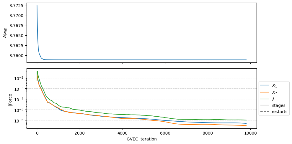
As with the tokamak case, we can extract and plot the history of the GVEC run to see the change in total MHD energy and the norm of the forces.

fig = run.plot_diagnostics_minimization()

---

Post-processing

Loading the state

As usual we load a gvec.State(🌐) so that we can evaluate and visualise the quantities we want.

state = run.state
# alternatively:
# state = gvec.find_state(runpath)

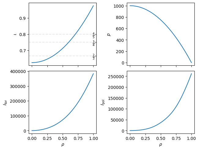
Visualize profiles

• First we plot the relevant profiles, now over the radial coordinate \(\rho\sim \sqrt{\Phi}\)

• The rotational transform and pressure are input profiles, and the current profiles are computed from the equilibrium solution.

We use the convenience plotting function plot_radial_profile(🌐), which computes the requested variables from the state.

# === Profiles === #
fig, axs = state.plot_radial_profile()

WARNING Computation of `I_pol` uses `rho=1.000000e-04` instead of the magnetic axis.

Visualize axis quantities

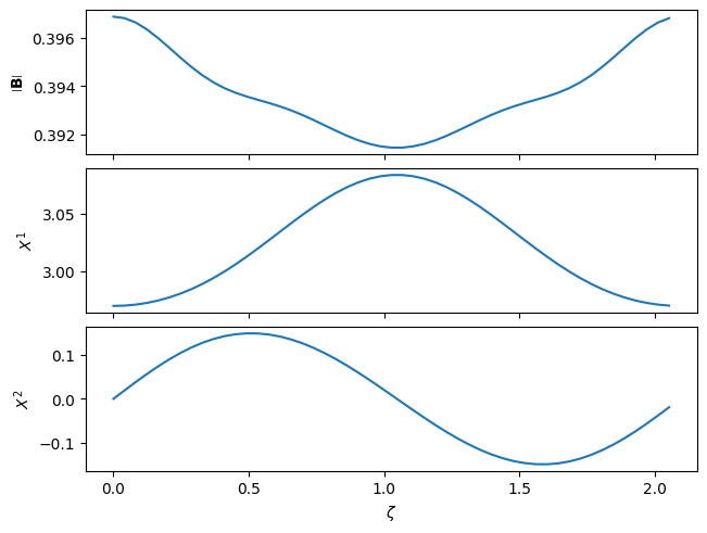
Let us now plot the magnetic field strength on axis and the axis position. Here \(X^1\) and \(X^2\) are equivalent to the cylindrical coordinates \(R,Z\) respectively.

Also here, we use a convenience plotting function plot_on_axis(🌐), which computes the requested variables from the state.

fig, axs = state.plot_on_axis(
    ["mod_B", "X1", "X2"], subplot_grid=[3, 1]
)

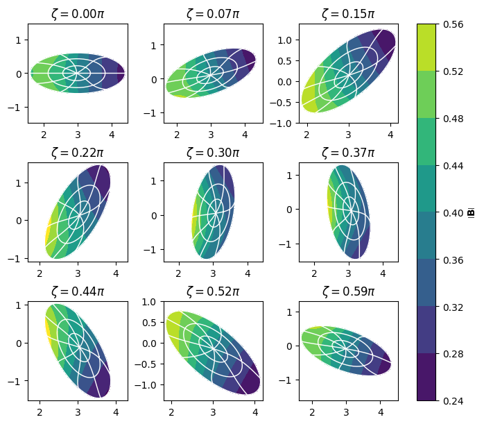
Plotting poloidal planes

We can also plot the magnetic field strength \(|B|\) on a series of poloidal planes, where we also show the flux surface geometry with contours of \(\rho\) and \(\theta_P\).

A convenience plotting function plot_poloidal_plane(🌐) is used here.

fig, axs = state.plot_poloidal_plane(plot_kwargs={"figsize": (8, 6)})

Evaluating equilibrium quantities

We will now extract two data sets for plotting, using state.evaluate(🌐). The first is the position of the magnetic axis \((\rho=0)\) on the full torus, and \(|B|\) along the axis.

Note derived quantities (such as \(|B|\)) cannot be evaluated exactly on the axis, so here we specify \(\rho=10^{-8}\).

ev_axis = state.evaluate(
    "pos",
    "N_FP",
    "mod_B",
    rho=[1.0e-8],
    theta=[0.0],
    zeta=np.linspace(0, 2 * np.pi, 201),
)

# reduce the xarray dataset 1D
ev_axis_1d = ev_axis.sel(rho=ev_axis.rho[0]).sel(
    theta=ev_axis.theta[0]
)

The second dataset is the full 3D volume on a single field period. Note that:

• It is possible to evaluate additional quantities that were not included initially in varlist.

• Previously evaluated quantities in the ev dataset are kept, and only the additional ones are.

# poloidal visualization points
theta = np.linspace(0, 2 * np.pi, 50)
# toroidal visualization points
zeta = np.linspace(0, 2 * np.pi / state.nfp, 8 * 4 + 1)
varlist = ["pos", "mod_B", "iota", "p", "I_tor", "I_pol"]

ev = state.evaluate(*varlist, rho=20, theta=theta, zeta=zeta)

# compute additional quantities
state.compute(ev, "grad_rho", "grad_theta", "grad_zeta");

WARNING Computation of `I_pol` uses `rho=1.000000e-04` instead of the magnetic axis.

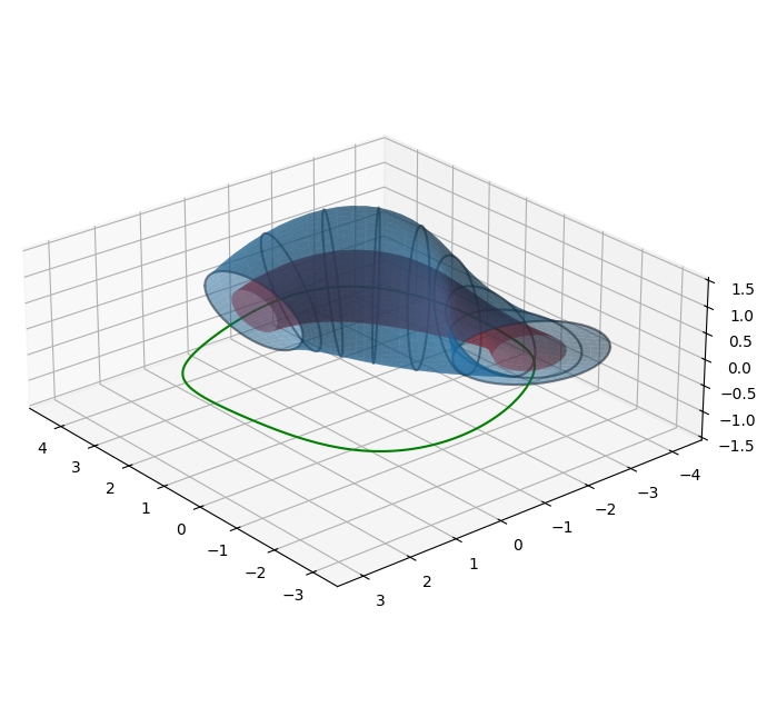
Custom 3D visualization

While we could also use the state.plot_3d_surface(🌐) method for 3D visualization, we will instead create a custom 3D visualization with matplotlib, showing two flux surfaces, boundary cuts and the magnetic axis. We first generate the data we want to visualize:

# axis position, reduced to a 1D array
ev_axis = state.evaluate(
    "pos",
    rho=1.0e-8,
    theta=0.0,
    zeta=np.linspace(0, 2 * np.pi, 201),
).squeeze()

# poloidal visualization points
theta = np.linspace(0, 2 * np.pi, 50)
# toroidal visualization points
zeta = np.linspace(0, 2 * np.pi / state.nfp, 8 * 4 + 1)

ev = state.evaluate("pos", rho=20, theta=theta, zeta=zeta)

x, y, z = np.asarray(ev.pos)

fig = plt.figure(figsize=(8, 8))
ax = fig.add_subplot(111, projection="3d", alpha=0.9)
# last surface in rho
ax.plot_surface(x[-1, :, :], y[-1, :, :], z[-1, :, :], alpha=0.5)
# cuts of the boundary
for iz in range(0, ev.sizes["tor"], 4):
    ax.plot3D(
        x[-1, :, iz], y[-1, :, iz], z[-1, :, iz], alpha=0.5, color="k"
    )
# flux surface mid-radius
x, y, z = np.asarray(ev.pos.sel(rho=0.5, method="nearest"))
ax.plot_surface(x, y, z, alpha=0.5, color="red")

x, y, z = np.asarray(ev_axis.pos)
ax.plot3D(x, y, z, color="green")

ax.set(aspect="equal")
ax.view_init(25, 140, 0)

Exporting data for visualization

For 3D visualizations one might want to change to powerful 3D visualization tools such as paraview. For such purposes pyGVEC datasets can easily be exported to the .vts format via the ev2vtk function. Note that all variables will be broadcast to the 3D grid defined by the pos variable. Hence, it might be advisable to select just those variables which will be used during the visualization to avoid unnecessary large files.

# compute additional quantities and add them to 'ev'
state.compute(ev, "p", "X1", "X2", "LA", "B");

from gvec.vtk import ev2vtk

variables_for_3D = ["X1", "X2", "LA", "pos", "B", "p"]
visu_data_3D = ev[variables_for_3D]
ev2vtk("pyGVEC_3d_visu", visu_data_3D)

xarray datasets can also be exported as netCDF (or a number of other file formats):

visu_data_3D.to_netcdf("pyGVEC_3d_visu.nc")

Note that you can output the paraview file from the command line by running

pygvec to-paraview

Use --help argument for details.