Coordinate conventions

GVEC coordinates

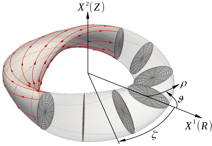
Sketch of the GVEC logical coordinate directions \(\rho,\vartheta,\zeta\) in a stellarator geometry (with magnetic field lines shown in red).

GVEC uses a flux aligned coordinate system with a radial coordinate \(\rho\in[0,1]\), proportional to the square root of the normalized toroidal flux, and two angular coordinates \(\vartheta,\zeta\in[0,2\pi]\). The Boozer-straight-fieldline-angles \(\vartheta_B,\zeta_B\in[0,2\pi]\) are a different set of flux aligned coordinates.

GVEC uses right-handed \((\rho,\vartheta,\zeta)\) and \((\rho,\vartheta_B,\zeta_B)\) systems with the poloidal angles \(\vartheta,\vartheta_B\) increasing counter-clockwise in the poloidal plane (of constant \(\zeta\) or \(\zeta_B\)). GVEC also uses a right-handed \((X^1,X^2,\zeta)\) reference coordinate frame, e.g. a cylindrical coordinate system \((R,Z,\zeta)\). Note that this definition of the cylindrical coordinate system has the toroidal angle \(\zeta\) increasing clockwise when viewing the \(R,Z\)-plane from above. For a curve-following G-Frame, \(\zeta\) can increase in any direction.

VMEC uses a \((R,\zeta,Z)\) reference frame with \(\zeta\) increasing counter-clockwise when viewed from above. If \(\vartheta\) is still increasing counter-clockwise in the poloidal plane, then the \((\rho,\vartheta,\zeta)\) coordinates in VMEC are left-handed. Some versions of VMEC also allow \(\vartheta\) increasing clockwise. To compare GVEC and VMEC, care must be taken to change the direction of the toroidal angle and associated quantities. DESC similarily defines \(\zeta\) increasing counter-clockwise and \(\vartheta\) increasing clockwise to obtain a right-handed system.

Different conventions

Assuming another code uses flux aligned coordinates \((s,u,v)\) with different conventions, i.e.

\(\qquad s=s(\rho)\,, \quad u=u(\vartheta)\,, \quad v=v(\zeta)\quad\) or

\(\qquad s=s(\rho)\,, \quad u=u(\vartheta_B)\,, \quad v=v(\zeta_B)\,.\)

In the following we will assume logical flux aligned coordinates \((\rho,\vartheta,\zeta)\), but the same formulas apply if one replaces \(\vartheta,\zeta\) by Boozer straight-fieldline-angles \(\vartheta_B,\zeta_B\).

From the relations \(s(\rho), u(\vartheta)\) and \(v(\zeta)\) we get the derivatives \(\frac{ds}{d\rho},\frac{du}{d\vartheta},\frac{dv}{d\zeta}\).

Geometric Quantities

reciprocal basis vectors

\[\begin{split} \begin{align} \boldsymbol{e}_s &:=\frac{\partial\boldsymbol{x}}{\partial s} & &= \left(\frac{ds}{d\rho}\right)^{-1} \boldsymbol{e}_\rho \\ \boldsymbol{e}_u &:=\frac{\partial\boldsymbol{x}}{\partial u} & &= \left(\frac{du}{d\vartheta}\right)^{-1} \boldsymbol{e}_\vartheta \\ \boldsymbol{e}_v &:=\frac{\partial\boldsymbol{x}}{\partial v} & &= \left(\frac{dv}{d\zeta}\right)^{-1} \boldsymbol{e}_\zeta \end{align} \end{split}\]

contravariant components of a vector \(\boldsymbol{Q}\)

\[\begin{split} \begin{align} Q^{s} &= \frac{ds}{d\rho} Q^{\rho} \\ Q^{u} &= \frac{du}{d\vartheta} Q^{u} \\ Q^{v} &= \frac{dv}{d\zeta} Q^{\zeta} \end{align} \end{split}\]

Jacobian determinant

\[ \mathcal{J} :=\boldsymbol{e}_{s}\cdot\boldsymbol{e}_{u}\times\boldsymbol{e}_{\zeta} = \left(\frac{ds}{d\rho}\frac{du}{d\vartheta}\frac{dv}{d\zeta}\right)^{-1} \mathcal{J}_{\rho\vartheta\zeta} \]

components of the metric tensor

\[\begin{split} \begin{align} g_{ss} &:=\boldsymbol{e}_{s}\cdot\boldsymbol{e}_{s} &&= \left(\frac{ds}{d\rho}\right)^{-2} g_{\rho\rho} \\ g_{su} &&&= \left(\frac{ds}{d\rho}\frac{du}{d\vartheta}\right)^{-1} g_{\rho\vartheta} \\ g_{sv} &&&= \left(\frac{ds}{d\rho}\frac{dv}{d\zeta}\right)^{-1} g_{\rho\zeta} \\ g_{uu} &&&= \left(\frac{du}{d\vartheta}\right)^{-2} g_{\vartheta\vartheta} \\ g_{uv} &&&= \left(\frac{du}{d\vartheta}\frac{dv}{d\zeta}\right)^{-1} g_{\vartheta\zeta} \\ g_{vv} &&&= \left(\frac{dv}{d\zeta}\right)^{-2} g_{\zeta\zeta} \end{align} \end{split}\]

components of the second fundamental form (of the fluxsurfaces)

\[\begin{split} \begin{align} \mathrm{II}_{uu} &:= \boldsymbol{n}\cdot\frac{\partial^{2}\boldsymbol{x}}{\partial u^{2}} &&= \left(\frac{du}{d\vartheta}\right)^{-2} \mathrm{II}_{\vartheta\vartheta} \\ \mathrm{II}_{uv} &&&= \left(\frac{du}{d\vartheta}\frac{dv}{d\zeta}\right)^{-1} \mathrm{II}_{\vartheta\zeta} \\ \mathrm{II}_{vv} &&&= \left(\frac{dv}{d\zeta}\right)^{-2} \mathrm{II}_{\zeta\zeta} \end{align} \end{split}\]