Theory

GVEC is already providing stellarator-type equilibrium solutions to the gyro-kinetic code GENE-3D [NMP+20],[MND+20],[WNM+21], the linear MHD stability code CASTOR-3D [PDS+23] and the nonlinear time-dependent MHD code JOREK-3D [NRH+22]. The new G-Frame feature and its application are presented in [HPM25] and [PDR+25].

GVEC builds upon the ideas of the well-established VMEC [HW83].

Continuous problem

To detail the continuous problem, we first introduce the total MHD energy in a domain \(\Omega\)

(1)\[\begin{align}\label{eq:W_MHD} W_\text{MHD} = \int_\Omega \frac{|\vec{B}|^2}{2\mu_0} + \frac{p}{(\gamma - 1)} \,\mathrm{d} x, \end{align}\]

with magnetic field \(\vec{B}\), pressure \(p\) and the ratio of specific heats \(\gamma\).

First, under the assumption of closed nested surfaces, the geometry is defined by an embedding map

(2)\[\begin{equation} f: (\rho,\thet,\zeta) \mapsto (x,y,z)\,, \label{eq:fmap} \end{equation}\]

where \((x,y,z)=:\vec{x} \in\R^3\) are Cartesian coordinates and \((\rho,\thet,\zeta)\in[0,1]\times[0,2\pi)\times[0,2\pi)\) are the logical coordinates in radial and angular directions.

The derivatives of \(f\) give the usual tangent basis vectors

(3)\[\begin{equation}\label{eq:covariant basis vectors} \erho =\pdv{\vec{x}}{\rho}\,,\quad \ethet =\pdv{\vec{x}}{\thet}\,,\quad \ezeta =\pdv{\vec{x}}{\zeta}\,. \end{equation}\]

We deduce the Jacobian determinant of \(f\) as

(4)\[\begin{equation}\label{eq:Jacobian} \Jac = \erho\cdot(\ethet\times\ezeta)\,, \end{equation}\]

the reciprocal basis vectors

(5)\[\begin{equation} \label{eq:contravariant basis vectors} \grad\rho = \left(\ethet\times\ezeta\right)\Jac^{-1}\,,\quad \grad\thet = \left(\ezeta\times\erho\right)\Jac^{-1}\,,\quad \grad\zeta = \left(\erho\times\ethet\right)\Jac^{-1}\,, \end{equation}\]

and the metric tensor

(6)\[\begin{equation}\label{eq:metric tensor} g_{\alpha\beta}=\vec{e}_{\alpha}\cdot\vec{e}_{\beta} \end{equation}\]

with \(\alpha,\beta\in\{\rho,\thet,\zeta\}\). It also follows that

(7)\[\begin{equation}\label{eq:from grad to e} \erho=\left(\grad\thet\times\grad\zeta\right)\Jac\,,\quad \ethet=\left(\grad\zeta\times\grad\rho\right)\Jac\,,\quad \ezeta=\left(\grad\rho\times\grad\thet\right)\Jac\,. \end{equation}\]

This allows us to write the MHD energy functional as

(8)\[\begin{equation} W_\text{MHD} = \rint\dblint \frac{1}{2\mu_0} (B^\alpha g_{\alpha\beta} B^\beta)\Jac + \frac{p}{(\gamma - 1)} \Jac\,\mathrm{d} \rho\,\mathrm{d}\thet\,\mathrm{d}\zeta. \end{equation}\]

with the covariant components \(B^\alpha=\vec{B}\cdot\grad\alpha\), and using Einstein summation convention, summing over repeated indices.

In the following, we first define the coordinates and the magnetic field \(\vec{B}\), to be able to write the MHD energy functional in terms of the solution variables.

Coordinate maps

Before we introduce the magnetic field representation, we begin with details on the coordinate systems.

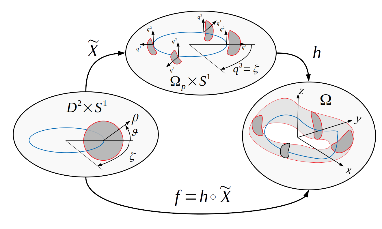
Illustration of logical and Cartesian coordinates and the coordinate transforms in GVEC. The logical domain with \((\rho,\thet,\zeta)\) coordinates is described by the unit disc, \(D^2\), and unit circle, \(S^1\), respectively. We assume a mapping \(\widetilde{X}\) from the logical domain to a toroidal domain \(\Omega_p\times S^1\), described by \((q^1,q^2)\) coordinates. Then, \(h\) maps from \((q^1,q^2,\zeta)\) to Cartesian coordinates \((x,y,z)\) of the real space domain \(\Omega\), as illustrated on the right.

As illustrated in the Figure above, the full map \(f:= h\circ \tilde{X}\) is decomposed into two maps,

(9)\[\begin{align} \tilde{X} &: (\rho,\thet,\zeta)\mapsto (q^1,q^2,q^3) = \big(X^1(\rho,\thet,\zeta),X^2(\rho,\thet,\zeta),\zeta\big) \\ h &: (q^1,q^2,q^3) \mapsto (x,y,z)=h(q^1,q^2,q^3) \end{align}\]

leaving \(X^1,X^2\) as functions of \((\rho,\thet,\zeta)\) to describe the geometry of each cross-section along \(\zeta\). The map \(h\) is fixed throughout the equilibrium calculation and can be specified by the user.

Simple examples of \(h\) are given by the periodic cylinder \((x,y,z) := (q^1,q^2,\zeta)\) and the conventional cylindrical representation \((x,y,z) := (q^1 \cos(\zeta),-q^1 \sin(\zeta),q^2)\). A new possibility for \(h\) is the G-Frame, a flexible coordinate frame which is moving along a closed curve and is fully user-defined, details are given in [HPM25].

It is always assumed that \((x,y,z) = h(q^1,q^2,q^3)\) is an orientation-preserving coordinate transformation, i.e., the Jacobian determinant is strictly positive, \(\det (Dh) > 0\). (Here and in the following \(D\) denotes the derivative operator.) For the composition \(f = h \circ \tilde{X}\) to be defined, the function \(\tilde{X}\) must take values in the domain of definition of \(h\). This is the only constraint that links \(h\) and \(\tilde{X}\). In addition, we require (independently of \(h\)) that

\[\begin{equation*} \det D\tilde{X} = \left(\partial_\rho X^1 \partial_\thet X^2 - \partial_\rho X^2 \partial_\thet X^1\right) > 0, \quad \text{for $\rho > 0$}, \end{equation*}\]

which is the Jacobian of the transformation \((\rho,\thet) \mapsto (X^1,X^2)\). Hence, for any fixed angle \(\zeta\), the map \((q^1, q^2) = \big(X^1(\rho,\thet,\zeta), X^2(\rho,\thet,\zeta)\big)\) is an orientation-preserving diffeomorphism from the unit disk, parametrized by polar coordinates \((\rho,\thet)\), into a domain in the \((q^1,q^2)\)-plane. By the chain rule, \(Df = Dh(\tilde{X}) D\tilde{X}\), we have that \(f\) is an orientation-preserving diffeomorphism away from the polar singularity at \(\rho=0\).

As the full map \(f\) is decomposed into \(f=h\circ \tilde{X}\), the Jacobian and metric terms are equally decomposed and computed as

(10)\[\begin{equation}\label{eq:Jac_h} \Jac=\Jac_h\Jac_p\,,\quad \Jac_h := \pdv{\vec{x}}{q^1}\cdot\left(\pdv{\vec{x}}{q^2}\times\pdv{\vec{x}}{q^3}\right)\,,\quad \Jac_p:=\left(\pdv{X^1}{\rho}\pdv{X^2}{\thet}-\pdv{X^2}{\rho}\pdv{X^1}{\thet}\right) \end{equation}\]

and

(11)\[\begin{equation}\label{eq:metric_h} g_{\alpha\beta}=\pdv{q^{i}}{\alpha}G_{ij}\pdv{q^{j}}{\beta}\,, \quad G_{ij}=\pdv{\vec{x}}{q^i}\cdot\pdv{\vec{x}}{q^j}\,, \end{equation}\]

with \((q^1,q^2,q^3):=(X^1,X^2,\zeta)\) and \(i,j=1,2,3\) and \(\alpha, \beta \in [\rho,\thet,\zeta]\).

A simple map: the torus

Sketch of the GVEC logical coordinate directions \(\rho,\vartheta,\zeta\) in a stellarator geometry (with magnetic field lines shown in red).

A widely used map for \(h\) is to map each cross-section \(q^1,q^2\) to \((R,Z)\) planes, as shown in the Figure above, which reads as

(12)\[\begin{equation}\label{eq:hmap torus} h:\quad (q^1,q^2,q^3)\mapsto(x,y,z):=(q^1\cos(q^3), -q^1\sin(q^3), q^2)\,. \end{equation}\]

Note that we have right-handed coordinate systems for both maps \(\tilde{X}\) and \(h\), requiring \(\Jac_p>0\) and \(\Jac_h>0\).

The Jacobian and metric tensor are simply \(\Jac_h=q^1\) and \(G_{ij}=\delta_{i1}\delta_{j1}+\delta_{i2}\delta_{j2}+\delta_{i3}\delta_{j3}(q^1)^2\).

The magnetic field

As described in [Hel14], [DHCS91], the magnetic field in flux coordinates is given as the curl of the vector potential

(13)\[\begin{align} \vec{B}&=\curl\vec{A}\,, \quad \vec{A} = \Phi\grad\thet^\star - \chi\grad\zeta^\star\,\\ \vec{B} &= \grad\Phi\times\grad\thet^\star - \grad\chi\times\grad\zeta^\star\,, \end{align}\]

with the toroidal magnetic flux \(\Phi\), the poloidal magnetic flux \(\chi\) and the straight field line angles \(\thet^\star\) and \(\zeta^\star\). However, the straight-field line angles are a result of the equilibrium solution and therefore not known a priori. Thus, we introduce an additional periodic function \(\lambda\), which maps the straight field line angles \((\thet^\star=\thet+\lambda(\rho,\thet,\zeta),\zeta^\star=\zeta)\) to general flux coordinates.

Note that the toroidal angle \(\zeta\) is fixed by the map \(h\), the boundary geometry then defines an arbitrary angular parameterization in \(\thet\), so that \(\lambda\) is free to set the straight field line angle \(\thet^\star\) at the boundary. Moreover, the magnetic fluxes are provided as inputs to the problem, and depend only on the flux surface label \(\rho\). With that in mind, the magnetic field is given as

(14)\[\begin{align} \vec{B} &=\Phi^\prime\nabla \rho \times \nabla(\thet+\lambda) - \chi^\prime\nabla \rho \times \nabla \zeta \\ &= \Phi^\prime \left(1+\partial_\thet\lambda\right) \nabla \rho \times \nabla \thet + \left(\chi^\prime - \Phi^\prime\partial_\zeta\lambda\right)\nabla \zeta \times \nabla \rho\,, \end{align}\]

where the prime indicates the derivative with respect to \(\rho\). Finally, we express the magnetic field into the two contravariant components and the tangent basis vectors in tangential direction of the flux surface,

(15)\[\begin{equation}\label{eq:magnetic field} \vec{B} = \frac{1}{\Jac}\left(b^\thet \ethet + b^\zeta \ezeta\right)\,,\quad b^\thet = \chi^\prime -\Phi^\prime\partial_\zeta\lambda\quad b^\zeta = \Phi^\prime(1+\partial_\thet\lambda)\,, \end{equation}\]

The MHD energy functional

In the previous sections, we have defined everything to be able to write the continuous MHD energy functional in terms of our unknowns \(u:= (X^1, X^2, \lambda)\).

(16)\[\begin{align}\label{eq:MHD energy functional expanded} W(u) &= \rint \dblint \left( -p(\rho)\Jac + \frac{1}{2\mu_0} \frac{(b^\alpha g_{\alpha\beta} b^\beta)}{\Jac} \right) \, \,\mathrm{d}\rho\,\mathrm{d}\thet\,\mathrm{d}\zeta, \end{align}\]

where we now fixed \(\gamma=0\), again use Einstein summation convention, but \(\alpha,\beta\in\{\thet,\zeta\}\) only.

First variation of the energy functional

Consider the test set of test functions \(v:=(Y^1(\rho,\thet,\zeta),Y^2(\rho,\thet,\zeta),\Lambda(\rho,\thet,\zeta))\), variations in the energy functional are then computed as

(17)\[\begin{align} -\operatorname{D} W(u) v &= \rint\dblint p(\rho)[\delta J] - \frac{1}{2\mu_0} [\delta L_B] \,\mathrm{d}\rho\,\mathrm{d}\thet\,\mathrm{d}\zeta \end{align}\]

where the variation of the magnetic energy term is

(18)\[\begin{align} [\delta L_B] = \frac{1}{\Jac} \left( b^\alpha b^\beta [\delta g_{\alpha \beta}] + 2g_{\alpha\beta} b^\alpha [\delta b^\beta] - \frac{b^\alpha g_{\alpha \beta} b^\beta }{\Jac} [\delta \Jac] \right) \end{align}\]

and terms related to the variation in \(X^1,X^2\) are

(19)\[\begin{align} [\delta \Jac]_{Y^1} &= \Jac_h \left(\pdv{X^2}{\thet}\pdv{Y^1}{\rho} - \pdv{X^2}{\rho} \pdv{Y^1}{\thet} \right) + \Jac_p \left( \pdv{\Jac_h}{q^1} Y^1 \right)\,, \\ [\delta \Jac]_{Y^2} &= \Jac_h \left(\pdv{X^1}{\rho} \pdv{Y^2}{\thet} - \pdv{X^1}{\thet}\pdv{Y^2}{\rho} \right) + \Jac_p \left( \pdv{\Jac_h}{q^2} Y^2 \right)\,, \end{align}\]

and

(20)\[\begin{align} [\delta g_{\alpha \beta}]_{Y^1} &= \pdv{q^i}{\alpha} G_{i1} \pdv{Y^1}{\beta} + \pdv{q^j}{\beta} G_{1j} \pdv{Y^1}{\alpha} + \left( \pdv{q^i}{\alpha} \pdv{G_{ij}}{q^1} \pdv{q^j}{\beta} \right) Y^1\,,\\ [\delta g_{\alpha \beta}]_{Y^2} &= \pdv{q^i}{\alpha} G_{i2} \pdv{Y^2}{\beta} + \pdv{q^j}{\beta} G_{2j} \pdv{Y^2}{\alpha} + \left( \pdv{q^i}{\alpha} \pdv{G_{ij}}{q^2} \pdv{q^j}{\beta} \right) Y^2\,, \end{align}\]

with \(i,j\in\{1,2,3\}\) and \((q^1,q^2,q^3)=(X^1,X^2,\zeta)\) as well as \(\alpha, \beta\in\{\thet,\zeta\}\).

The terms related to the variation in \(\lambda\) are

(21)\[\begin{equation} [\delta b^\thet]_\Lambda = \Phi^\prime \pdv{\Lambda}{\zeta}, \qquad [\delta b^\zeta]_\Lambda = -\Phi^\prime \pdv{\Lambda}{\thet}. \end{equation}\]

We can collect the terms corresponding to the derivative of each component to obtain,

(22)\[\begin{align}\label{eq:energy functional derivative lambda terms} -\operatorname{D}_\lambda W(u) \Lambda = \rint\dblint \frac{\Phi^\prime}{\mu_0\Jac} b^\alpha \left(- g_{\alpha\zeta}\pdv{\Lambda}{\thet} + g_{\alpha\thet}\pdv{\Lambda}{\zeta} \right) \,\mathrm{d}\rho\,\mathrm{d}\thet\,\mathrm{d}\zeta \end{align}\]

and for \(k\in\{1,2\}\),

(23)\[\begin{align}\label{eq:energy functional derivative X terms} -\operatorname{D}_{X^k} W(u) Y^k = \rint\dblint \left( p(\rho) + \frac{b^\alpha g_{\alpha\beta} b^\beta}{2\mu_0\Jac^2} \right) [\delta \Jac]_{Y^k} - \frac{1}{2\mu_0} \frac{b^\alpha b^\beta}{\Jac} [\delta g_{\alpha\beta}]_{Y^k} \,\mathrm{d}\rho\,\mathrm{d}\thet\,\mathrm{d}\zeta. \end{align}\]

Discretization

For simplicity, we explain the discretization using a placeholder scalar unknown \(U(\rho,\thet,\zeta)\), that can be any of the solution variables \(X^1(\rho,\thet,\zeta),X^2(\rho,\thet,\zeta),\lambda(\rho,\thet,\zeta)\). \(U\) is discretised by a tensor-product of B-splines in the radial direction \(\rho\) and a double-angle Fourier series in poloidal and toroidal angles \((\thet,\zeta)\)

(24)\[\begin{equation} U(\rho,\thet,\zeta) = \sum_{k=1}^{k\submax} \sum_{\ell=\ell\submin}^{\ell\submax} \hat{U}_{k,\ell} \rbasis_k(\rho) \fbasis_\ell(\thet,\zeta) \end{equation}\]

with coefficients \(\hat{U}_{k,\ell}\), B-Spline basis functions \(\rbasis_k(\rho)\) and Fourier basis functions \(\fbasis_\ell(\thet,\zeta)\).

The double-angle Fourier series is defined by the maximum mode numbers \((m\submax,n\submax)\) in poloidal and toroidal direction. The toroidal mode number on the full torus (\(\zeta=[0,2\pi]\)) is a product of the Fourier mode number \(n\) on one field period and the number of field periods \(\nfp\). We write all Fourier basis functions \(\fbasis_\ell(\thet,\zeta)\) as a list of length \(\ell\submax=(m\submax+1)(2n\submax+1)\),

(25)\[\begin{equation} \begin{aligned} \left\{\fbasis_\ell(\thet,\zeta)\right\}_{\ell=1}^{\ell\submax} =\Big\{&1,\left\{\cos(-n\nfp\zeta), n=1,\dots,n\submax\right\},\\ &\left\{\cos(m\thet-n\nfp\zeta), m=1,\dots,m\submax,\,n=-n\submax,\dots,n\submax\right\},\\ &\left\{\sin(-n\nfp\zeta), n=1,\dots,n\submax\right\}, \\ &\left\{\sin(m\thet-n\nfp\zeta), m=1,\dots,m\submax,\,n=-n\submax,\dots,n\submax\right\}\Big\}\,. \end{aligned} \end{equation}\]

The mode number \(m,n\) can be deduced from the index \(\ell\).

To impose stellarator symmetry [DH98], we restrict the list of Fourier basis functions to a subset of either cosines, using \(\ell\submin=1,\ell\submax=m\submax(2n\submax+1)+n\submax+1\), or sines, using \(\ell\submin=m\submax(2n\submax+1)+n\submax+2,\ell\submax=(m\submax+1)(2n\submax+1)\). (In cylinder coordinates, stellarator symmetry implies \(R(\thet,\zeta)=R(-\thet,-\zeta)\) and \(Z(\thet,\zeta)=-Z(-\thet,-\zeta)\), thus cosine for \(R\) and sine for \(Z\).)

The B-Spline in \(\rho\) is defined by the polynomial degree \(p\) and a set of grid points \(\{\rho_i\}_{i=1}^{N_r}\) with \(\rho_1=0,\rho_{N_r}=1\). From the grid points, a knot sequence is constructed, with a multiplicity of \(p+1\) at the first and the last knot. As we do not allow for any multiplicity of internal knots, the continuity of the B-Spline is \(p-1\) and the number of basis functions is \(k\submax=N_r+(p-1)\).

Note that all variables \(X^1,X^2,\lambda\) share the same radial grid, but are allowed to have different polynomial degrees of the B-Spline.

Boundary conditions in radial direction

The first and last B-Spline coefficient equals the value at the boundary. This allows to easily set Dirichlet boundary conditions. As we only consider fixed-boundary equilibria in this work, we impose a Dirichlet boundary condition at \(\rho=1\) for the variables \(X^1,X^2\), by setting the last B-Spline coefficient of each Fourier modes to the value provided by the boundary geometry. For \(\lambda\), no boundary condition is imposed at \(\rho=1\), as its boundary value is an unknown of the solution.

We know from the mapping \(\widetilde{X}\) (see Coordinate maps) that each cross-section \(X^1(\rho,\thet,\zeta=\text{const.})\), \(X^2(\rho,\thet,\zeta=\text{const.})\) represents a map to the unit disc \(\rho\exp(\mathrm{i}\thet)\), which has to be smooth at any point inside the unit disc. Away from the singular point \(\rho=0\), the tensor-product of B-Splines and Fourier series is smooth, up to the polynomial degree of the B-Spline.

In order to preserve the same smoothness at the magnetic axis \(\rho=0\), we need to impose a boundary condition for the B-Spline representation of each Fourier mode that depends on the poloidal mode number \(m\). The necessary and sufficient conditions for smoothness at the magnetic axis have been presented in [LB90].

First, the value of \(U\) at \(\rho=0\) must be unique and independent of \(\thet\), thus it is determined solely by the B-Spline representing the \(m=0\) poloidal mode. All B-Splines representing non-zero poloidal modes have zero Dirichlet boundary condition at \(\rho=0\).

Additionally, the boundary condition must involve radial derivatives of the B-Spline, up to the polynomial degree \(p\). The argument in [LB90] is that on the unit disc, a polynomial of degree \(m\) can be expressed \((\rho\exp(\mathrm{i}\thet))^m=\rho^m\exp(\mathrm{i}m\thet)\). Hence, for a poloidal mode \(f(\rho)\mathrm{e}^{\mathrm{i}m\thet}\), the radial function \(f(\rho\to 0)\) must exclude terms \(\rho^j\) where \(j<m\), in order to be smooth. Hence, we have to impose that all radial derivatives \(<m\) must vanish

(26)\[\begin{equation} \left.\pdv[j]{U}{\rho}\right|_{\rho=0}=0,\quad\forall j<m \end{equation}\]

Note that poloidal modes with \(m\geq p\) do not have a contribution to the solution \(U\) at \(\rho=0\).

Finally, the boundary condition needs to impose symmetry for even poloidal modes

(27)\[\begin{equation} m\quad\text{even}:\qquad \left.\pdv[j]{U}{\rho}\right|_{\rho=0}=0, \quad \forall j\quad \text{odd}\,, \end{equation}\]

and anti-symmetry for odd poloidal modes

(28)\[\begin{equation} m \quad\text{odd}:\qquad \left.\pdv[j]{U}{\rho}\right|_{\rho=0}=0, \quad\forall j\quad \text{even}\,. \end{equation}\]

The boundary condition at the axis results in a smoothness constraint that is imposed on all variables \(X^1,X^2\) and \(\lambda\). Here is an explicit example of all boundary conditions set at the axis, for a B-Spline of degree \(p=5\) and \(m\submax=6\) poloidal modes:

\[\begin{align*} &m=0: &\left.\pdv[j]{U}{\rho}\right|_{\rho=0}&= 0, \quad j = 1, 3, 5 \\ &m=1: &\left.\pdv[j]{U}{\rho}\right|_{\rho=0}&= 0, \quad j = 0, 2, 4 \\ &m=2: &\left.\pdv[j]{U}{\rho}\right|_{\rho=0}&= 0, \quad j = 0, 1, 3, 5 \\ &m=3: &\left.\pdv[j]{U}{\rho}\right|_{\rho=0}&= 0, \quad j = 0, 1, 2, 4 \\ &m=4: &\left.\pdv[j]{U}{\rho}\right|_{\rho=0}&= 0, \quad j = 0, 1, 2, 3, 5 \\ &m=5: &\left.\pdv[j]{U}{\rho}\right|_{\rho=0}&= 0, \quad j = 0, 1, 2, 3, 4 \\ &m=6: &\left.\pdv[j]{U}{\rho}\right|_{\rho=0}&= 0, \quad j = 0, 1, 2, 3, 4, 5 \end{align*}\]

and for \(m>0\) the value at \(U(\rho=0)\) is also et to zero.

Approximation of the integrals

We approximate the integrals in \(\rho, \thet, \zeta\) by numerical quadrature.

(29)\[\begin{align} \rint \dblint W(\rho,\thet,\zeta) \,\mathrm{d}\rho\,\mathrm{d}\thet\,\mathrm{d}\zeta &= N_{FP}\rint \int\limits_{0}^{2\pi}\!\int\limits_{0}^{2\pi/N_{FP}} W(\rho,\thet,\zeta) \,\mathrm{d}\rho\,\mathrm{d}\thet\,\mathrm{d}\zeta, \\ &\approx \sum_{i=1}^{n_q} \omega_i \sum_{j=1}^{n_\thet} \sum_{k=1}^{n_\zeta} W(\rho^q_i,\thet_j,\zeta_k), \end{align}\]

where \(\omega_i\) is the quadrature weight and \(n_q\) is the total number of Gauss quadrature points in the radial direction. The total number is given by the number of grid elements of the B-Splines and the number of quadrature points in each B-Spline element, chosen to integrate piecewise-polynomial functions exactly up to degree \(2p+1\). The number of integration points in the poloidal and toroidal direction are \(n_\thet\), \(n_\zeta\) and we choose the positions as

\[\begin{equation*} \thet_j=2\pi\frac{j-1/2}{n_\thet}\,,\quad \zeta_k=\frac{2\pi}{\nfp}\frac{k-1/2}{n_\zeta}\,. \end{equation*}\]

We choose the number of integration points \(n_\thet\), \(n_\zeta\) \(4\) times larger than the maximum mode number in each direction.

An equation for lambda

While the degrees of freedom of \(\lambda(\rho,\thet,\zeta)\) are evolved in the minimization of the energy functional, an initial guess is required. One option is to simply choose \(\lambda(\rho,\thet,\zeta)=0\), however a better initial guess can be obtained by solving an elliptic equation for \(\lambda\).

In an ideal MHD equilibria we have the relations,

(30)\[\begin{align}\label{eq:nested current surface} \nabla p &= \vec{J}\times \vec{B}, \\ \vec{B} \cdot \nabla p = 0 &\iff \vec{B} \cdot \nabla \rho = 0, \label{eq:nested flux surface} \\ \mu_0 \vec{J} \cdot \nabla p = 0 &\iff \nabla \rho \cdot (\nabla\times\vec{B}) = 0. \end{align}\]

The equation states that \(\vec{B}\) and \(\vec{J}\) are tangent along a given flux surface labelled by \(\rho\), combining with the result from earlier gives \(J^\rho=0\), or

(31)\[\begin{align} \pdv{B_\zeta}{\thet} - \pdv{B_\thet}{\zeta} &= 0, \\ \pdv{\thet}\left( g_{\zeta\thet} B^\thet + g_{\zeta\zeta} B^\zeta \right) - \pdv{\zeta} \left( g_{\thet\thet} B^\thet + g_{\thet\zeta} B^\zeta \right) &= 0, \\ \pdv{\thet} \left( \frac{g_{\zeta\thet}}{\Jac} \, \left( \chi^\prime - \Phi^\prime \pdv{\lambda}{\zeta} \right) + \frac{g_{\zeta\zeta}}{\Jac} \, \Phi^\prime \left(1 + \pdv{\lambda}{\thet} \right) \right) & \\ \qquad\quad - \pdv{\zeta} \left( \frac{g_{\thet\thet}}{\Jac} \, \left( \chi^\prime - \Phi^\prime \pdv{\lambda}{\zeta} \right) + \frac{g_{\thet\zeta}}{\Jac} \, \Phi^\prime \left(1 + \pdv{\lambda}{\thet} \right) \right) &= 0. \end{align}\]

Rearranging slightly to isolate \(\lambda\) terms we arrive at,

\[\begin{equation*}\label{eq:lambda elliptic equation} \begin{aligned} &\Phi^\prime \left[ \pdv{\thet} \frac{1}{\Jac} \left( -g_{\zeta\thet} \pdv{\lambda}{\zeta} + g_{\zeta\zeta} \pdv{\lambda}{\thet} \right) - \pdv{\zeta} \frac{1}{\Jac} \left( -g_{\thet\thet} \pdv{\lambda}{\zeta} + g_{\thet\zeta}\pdv{\lambda}{\thet} \right) \right] = \\&\qquad\qquad - \left[ \pdv{\thet} \frac{1}{\Jac} \left( g_{\zeta\thet} \chi^\prime + g_{\zeta\zeta} \Phi^\prime\right) - \pdv{\zeta} \frac{1}{\Jac} \left( g_{\thet\thet} \chi^\prime + g_{\thet\zeta}\Phi^\prime \right) \right]. \end{aligned} \end{equation*}\]

By muliplying with the Fourier test function \(\fbasis(\thet,\zeta)\) and integrating over \(\thet\) and \(\zeta\) we obtain a weak equation for \(\lambda\) at a given \(\rho\),

(32)\[\begin{equation} \begin{aligned} &\Phi^\prime \dblint \frac{1}{\Jac} \left( \left( -g_{\thet\zeta} \pdv{\lambda}{\zeta} + g_{\zeta\zeta} \pdv{\lambda}{\thet} \right) \pdv{\fbasis}{\thet} - \left( -g_{\thet\thet} \pdv{\lambda}{\zeta} + g_{\thet\zeta} \pdv{\lambda}{\thet} \right) \pdv{\fbasis}{\zeta} \right) \;\dd\thet\;\dd\zeta = \\ &\qquad\qquad \dblint\frac{1}{\Jac} \left( ( g_{\thet\thet} \chi^\prime + g_{\thet\zeta} \Phi^\prime ) \pdv{\fbasis}{\zeta} - (g_{\zeta\thet} \chi^\prime + g_{\zeta\zeta} \Phi^\prime ) \pdv{\fbasis}{\thet} \right) \;\dd\thet\;\dd\zeta, \end{aligned} \end{equation}\]

where we have applied integration by parts to both sides. Finally, to facilitate the discretisation we rearrange the above equation to obtain,

(33)\[\begin{align}\label{eq:lambda elliptic equation weak form} \begin{aligned} & \dblint \frac{\Phi^\prime}{\Jac} \left( \left( g_{\zeta\zeta} \pdv{\fbasis}{\thet} - g_{\thet\zeta} \pdv{\fbasis}{\zeta} \right) \pdv{\lambda}{\thet} + \left( - g_{\thet\zeta} \pdv{\fbasis}{\thet} + g_{\thet\thet} \pdv{\fbasis}{\zeta} \right) \pdv{\lambda}{\zeta} \right) \dd{\thet}\dd{\zeta} \\&\qquad\qquad= \dblint \frac{1}{\Jac} \left( \chi^\prime \left( g_{\thet\thet} \pdv{\fbasis}{\zeta} - g_{\zeta\thet} \pdv{\fbasis}{\thet} \right) + \Phi^\prime \left( g_{\thet\zeta} \pdv{\fbasis}{\zeta} - g_{\zeta\zeta} \pdv{\fbasis}{\thet} \right) \right) \dd{\thet}\dd{\zeta}. \end{aligned} \end{align}\]

Solving the discrete equation

By taking the test function space the same as our solution space for lambda, we have,

(34)\[\begin{equation}\label{eq:discretised weak equation for lambda} \begin{aligned} \sum_j \Lambda^j &\dblint \frac{\Phi^\prime}{\Jac} \left( \left( g_{\zeta\zeta} \pdv{\fbasis^i}{\thet} - g_{\thet\zeta} \pdv{\fbasis^i}{\zeta} \right) \pdv{\fbasis^j}{\thet} + \left( - g_{\thet\zeta} \pdv{\fbasis^i}{\thet} + g_{\thet\thet} \pdv{\fbasis^i}{\zeta} \right) \pdv{\fbasis^j}{\zeta} \right) \dd\thet\,\dd\zeta \\=& \dblint \left( \frac{\chi^\prime}{\Jac} \left( g_{\thet\thet} \pdv{\fbasis^i}{\zeta} - g_{\zeta\thet} \pdv{\fbasis^i}{\thet} \right) + \frac{\Phi^\prime}{\Jac} \left( g_{\thet\zeta} \pdv{\fbasis^i}{\zeta} - g_{\zeta\zeta} \pdv{\fbasis^i}{\thet} \right) \right) \dd\thet\,\dd\zeta. \end{aligned} \end{equation}\]

Letting

(35)\[\begin{align} Q_\thet^i &= \dblint \frac{1}{\Jac} \left( g_{\thet\thet} \pdv{\fbasis^i}{\zeta} - g_{\zeta\thet} \pdv{\fbasis^i}{\thet} \right) \;\dd\thet\;\dd\zeta, \\ Q_\zeta^i &= \dblint \frac{1}{\Jac} \left( g_{\thet\zeta} \pdv{\fbasis^i}{\zeta} - g_{\zeta\zeta} \pdv{\fbasis^i}{\thet} \right) \;\dd\thet\;\dd\zeta, \end{align}\]

and finally write the discrete equation system as,

(36)\[\begin{align}\label{eq:lambda discrete elliptic equation compact} - \sum_j A^{ij}\Lambda^j &= \chi^\prime Q_\thet^i + \Phi^\prime Q_\zeta^i, \\ A^{ij} &= \Phi^\prime\left( Q_\thet^i \pdv{\fbasis^j}{\thet} + Q_\zeta^i \pdv{\fbasis^j}{\zeta} \right). \end{align}\]

Since \(A^{ij}\) arises from the elliptic equation, it follows that \(A^{ij}\) is a dense symmetric positive definite matrix.

Transformation to Boozer coordinates

For any straight-field line angles \(\thet^\star,\zeta^\star\), the following condition always holds

(37)\[\begin{align} \thet^\star-\iota(\rho)\zeta^\star = \text{const.} \label{eq:condSFL} \end{align}\]

with \(\iota(s)=\frac{\chi^\prime(\rho)}{\Phi^\prime(\rho)}\). We can change from one SFL coordinate to the other by adding a periodic function \(\nu\)

(38)\[\begin{align} \zeta^{\star}_2 &= \zeta^\star_1+ \nu(\rho,\thet,\zeta) \\ \thet^{\star}_2 &= \thet^\star_1+ \iota(\rho)\nu(\rho,\thet,\zeta) \end{align}\]

The natural SFL coordinates in GVEC (and VMEC) are PEST angles \(\thet_P,\zeta_P\), since we already know the transformation with \(\lambda\) from the VMEC angles \(\thet,\zeta\)

(39)\[\begin{equation} \thet^\star_P = \thet + \lambda(\rho,\thet,\zeta)\,,\qquad \zeta_P = \zeta \end{equation}\]

Then, we define the Boozer angles \(\thet_B,\zeta_B\) as

(40)\[\begin{equation} \thet^\star_B = \thet + \lambda(\rho,\thet,\zeta) + \iota(\rho)\nu(\rho,\thet,\zeta)\,,\qquad \zeta^\star_B = \zeta + \nu(\rho,\thet,\zeta) \end{equation}\]

The magnetic field in Boozer coordinates in contra-variant form

(41)\[\begin{equation} B = \Phi^\prime(\rho) \nabla \rho \times \nabla \thet^\star_B + \chi^\prime(\rho) \nabla \zeta^\star_B\times \nabla \rho \end{equation}\]

with the components

(42)\[\begin{align} B^{\thet^\star_B} &= B\cdot \nabla \thet^\star_B = \frac{\chi^\prime(\rho)}{\Jac_B}\,,\\ B^{\zeta^\star_B} &= B\cdot \nabla \zeta^\star_B = \frac{\Phi^\prime(\rho)}{\Jac_B}\,,\\ \frac{1}{\Jac_B} &= \nabla \rho\cdot(\nabla \thet^\star_B\times \nabla \zeta^\star_B) \end{align}\]

In addition, for Boozer coordinates, the angular components of the magnetic field in co-variant form become flux surface quantities as well:

(43)\[\begin{equation} B = \Btavg \nabla \thet^\star_B + \Bzavg \nabla \zeta^\star_B + X(\rho,\thet^\star_B,\zeta^\star_B) \nabla \rho \label{eq:Bcov_boozer} \end{equation}\]

with the averages being proportional to the toroidal and poloidal current profiles computed from the flux surface average at \(\rho\)

(44)\[\begin{equation} \Btavg = \frac{1}{4\pi^2}\dblint B_\thet d\thet d\zeta \,,\quad \Bzavg = \frac{1}{4\pi^2}\dblint B_\zeta d\thet d\zeta \end{equation}\]

If we insert the transformation,

(45)\[\begin{equation} \begin{aligned} B &= \Btavg \nabla (\thet+\lambda+\iota\nu) + \Bzavg \nabla (\zeta+ \nu) + X \nabla \rho \\ &= \left(\Btavg(1 + (\partial_\thet\lambda)) + (\iota \Btavg+\Bzavg)(\partial_\thet \nu)\right) \nabla \thet \\ &\quad + \left(\Bzavg +\Btavg (\partial_\zeta\lambda) + \left(\iota\Btavg+\Bzavg\right)(\partial_\zeta \nu)\right)\nabla \zeta \\ &\quad + \left(X+\Btavg (\partial_\rho\lambda) + \left(\iota\Btavg+\Bzavg\right)(\partial_\rho \nu)+\Btavg \nu (\partial_\rho \iota)\right) \nabla \rho \\ &= B_\thet \nabla \thet + B_\zeta \nabla \zeta + B_\rho \nabla \rho \end{aligned} \end{equation}\]

We can relate the components

(46)\[\begin{align} B_\thet &= \Btavg(1 + \partial_\thet \lambda) + (\iota\Btavg+\Bzavg)\partial_\thet \nu\,,\\ B_\zeta &= \Bzavg +\Btavg\partial_\zeta \lambda + (\iota\Btavg+\Bzavg)\partial_\zeta \nu \end{align}\]

and deduce

(47)\[\begin{align} \partial_\thet \nu &=\frac{B_\thet- \Btavg(1 + (\partial_\thet \lambda))}{(\iota\Btavg+\Bzavg)}\,,\\ \partial_\zeta \nu &= \frac{B_\zeta -\Bzavg -\Btavg(\partial_\zeta \lambda)}{(\iota\Btavg+\Bzavg)} \end{align}\]

Here one sees that the integrability condition \(\partial_\zeta(\partial_\thet \nu)-\partial_\thet(\partial_\zeta \nu)=0\) is only satisfied if \(\partial_\zeta(B_\thet)-\partial_\thet(B_\zeta)=0\), which is analogue to \(J^\rho=0\).

The calculation of \(\nu\) is simplified by defining \(\nu=\frac{\omega+\lambda}{(\iota\Btavg+\Bzavg)}\), so that the unknown becomes simply

(48)\[\begin{equation} \partial_\thet \omega=B_\thet- \Btavg\,,\quad \partial_\zeta \omega = B_\zeta -\Bzavg \end{equation}\]

We can compute the Fourier expansion of \(\omega=\sum_{m,n} \omega_{mn} \sigma_{mn}(\thet,\zeta)\), with \(\omega_{00}=0\) (assume here that \(\sigma_{mn}(\thet,\zeta)=e^{\mathrm{i}(m\thet-n\zeta)}\))

(49)\[\begin{equation} \begin{aligned} 2\pi^2\mathrm{i}m\omega_{mn} &= \dblint(B_\thet- \Btavg) \sigma_{mn} d\thet d\zeta \,,\quad \text{if} \quad m\neq 0 \\ -2\pi^2\mathrm{i}n\omega_{mn} &= \dblint(B_\zeta -\Bzavg)\sigma_{mn} d\thet d\zeta \,,\quad \text{if} \quad n\neq 0 \end{aligned} \end{equation}\]

which, for \(\sigma\) being either cos or sin base, leads to

(50)\[\begin{equation} \begin{aligned} \omega_{mn} &= \frac{1}{m}\frac{1}{2\pi^2} \dblint(B_\thet- \Btavg)\sigma_{mn} d\thet d\zeta \,,\quad \text{if} \quad m\neq 0 \\ \omega_{mn} &= \frac{-1}{n}\frac{1}{2\pi^2}\dblint(B_\zeta -\Bzavg)\sigma_{mn} d\thet d\zeta \,,\quad \text{if} \quad n\neq 0 \end{aligned} \end{equation}\]

with the norm of of each mode \(\sigma_{mn}(\thet,\zeta)=\sin(m\thet-n\zeta)/\cos(m\thet-n\zeta)\)

Now if the integrability condition would be satisfied, \(\omega_{mn}, m\neq 0,n\neq 0\), computed in the two ways must yield the same. The condition translates to

(51)\[\begin{equation} \begin{aligned} (\mathrm{i}m\omega_{mn})(-\mathrm{i}n) -(-\mathrm{i}n\omega_{mn})(\mathrm{i}m) &=0\\ \dblint\left(B_\thet- \Btavg\right) \partial_\zeta \sigma_{mn} - \left(B_\zeta -\Bzavg\right)\partial_\thet\sigma_{mn} d\thet d\zeta&=0\\ \dblint\left(B_\thet\partial_\zeta\sigma_{mn} - B_\zeta\partial_\thet\sigma_{mn}\right)d\thet d\zeta &=0 \end{aligned} \end{equation}\]

which results in the weak form of \(J^\rho=0\). Note that only if \(\lambda\) is recomputed from \(J^\rho=0\) (involving fluxes and the mapping), using the same basis functions as \(\omega\), one can guarantee the integrability condition of \(\nu\) to machine precision.

Computing \(|B|\) in Boozer coordinates

In Boozer coordinates \((\thet^\star_B,\zeta^\star_B)\), expressed in the usual GVEC coordinates \((\thet,\zeta)\) reads as

(52)\[\begin{equation} \begin{aligned} \thet^\star_B &= \thet + \lambda(\rho,\thet,\zeta)+\iota(s) \nu(\rho,\thet,\zeta)\,,\\ \zeta^\star_B &= \zeta + \lambda(\rho,\thet,\zeta)+ \nu(\rho,\thet,\zeta)\,.\\ \end{aligned} \end{equation}\]

The magnetic field strength is computed

(53)\[\begin{equation} |B|^2={B^{\thet^\star_B} B_{\thet^\star_B} + B^{\zeta^\star_B} B_{\zeta^\star_B}}=\frac{1}{\Jac_B}(\chi^\prime\Btavg-\Phi^\prime\Bzavg) \end{equation}\]

thus the variation on a flux surface only depends on \(1/\Jac_B\).

Recalling the mapping \(f:(\rho,\thet,\zeta)\mapsto(x,y,z)\), and introducing the mapping \(g: (\rho,\thet,\zeta)\mapsto(s,\thet^\star_B,\zeta^\star_B)\), and the mapping \(f^\star:(s,\thet^\star_B,\zeta^\star_B)\mapsto(x,y,z)\), its clear that \(f^\star=g^ {-1}\circ f\). Thus we find the Boozer Jacobian,

(54)\[\begin{equation} \begin{aligned} 1/\Jac_B(\thet,\zeta) &=:1/\det(f^\star)=\det(g)/\det(f) \\ &= \Jac(\thet,\zeta)^{-1}\left(\pdv{\thet^\star_B}{\thet}\pdv{\zeta^\star_B}{\zeta}-\pdv{\thet^\star_B}{\zeta}\pdv{\zeta^\star_B}{\thet}\right)\\ &= \frac{1}{\Jac(\thet,\zeta)}\left((1+\lambda_{,\thet}+\iota \nu_{,\thet})(1+\nu_{,\zeta})-(\lambda_{,\zeta}+\iota \nu_{,\zeta})\nu_{,\thet})\right) \end{aligned} \end{equation}\]

Other choices for hmap

As mentioned above, other choices of the hmap are available, besides the one of cylindrical coordinates:

(55)\[\begin{equation} h:\quad (q^1,q^2,q^3)\mapsto(x,y,z):=(q^1\cos(\zeta), -q^1\sin(\zeta),q^2)\,, \end{equation}\]

with the Jacobian and metric tensor \(\Jac_h=q^1\) and \(G_{ij}=\delta_{i1}\delta_{j1}+\delta_{i2}\delta_{j2}+\delta_{i3}\delta_{j3}\left(q^1\right)^2\).

Periodic Cylinder

We can also map to the periodic cylinder of length \(L_c\) with its axis pointing in \(y\) axis:

(56)\[\begin{equation} h:\quad (q^1,q^2,q^3)\mapsto(x,y,z):=(q^1, -\frac{L_c}{2\pi}\zeta,q^2)\,. \end{equation}\]

The Jacobian and metric tensor are simply \(\Jac_h=\frac{L_c}{2\pi}\) and \(G_{ij}=\delta_{i1}\delta_{j1}+\delta_{i2}\delta_{j2}+\delta_{i3}\delta_{j3}\left(\frac{L_c}{2\pi}\right)^2\).

The knot

As an example of non-standard choice of the map we construct coordinates based on the \((k,l)\)-torus. The map is a generalization of the standard cylindrical coordinates \((R,Z)\) given by

(57)\[\begin{equation} h:\quad (q^1,q^2,q^3)\mapsto(x,y,z):=(R_l(q^1,\zeta) \cos(k\zeta), -R_\ell(q^1,\zeta)\sin(k\zeta), Z_\ell(q^2,\zeta) )\,. \end{equation}\]

where \(k,l\) are coprime integers and

(58)\[\begin{align} R_\ell(q^1,\zeta) &= R_0 + \delta \cos(\ell\zeta) + q^1, \\ Z_\ell(q^2,\zeta) &= \delta \sin(\ell\zeta) + q^2, \end{align}\]

with \(R_0>0\) a positive radius, which plays the same role as the major radius, and \(\delta\) a real constant. The derivatives of the mapping are

(59)\[\begin{equation} Dh:\quad \pdv{\vec{x}}{q^1} = \left[ {\begin{array}{*{20}c} \cos(k\zeta)\\ -\sin(k\zeta) \\ 0 \end{array} } \right] \,,\quad \pdv{\vec{x}}{q^2} = \left[ {\begin{array}{*{20}c} 0\\ 0 \\ 1 \end{array} } \right] \,,\quad \pdv{\vec{x}}{q^3}= \left[ {\begin{array}{*{20}c} -H \\ -K \\ L \end{array} } \right] \end{equation}\]

where

(60)\[\begin{align} H &= kR_\ell \sin(k\zeta) + \ell \delta \sin(\ell\zeta) \cos(k\zeta), \\ K &= k R_\ell \cos(k\zeta) - \ell \delta \sin(\ell\zeta) \sin(k\zeta), \\ L &= \ell \delta \cos(\ell\zeta). \end{align}\]

The metric tensor amounts to

(61)\[\begin{equation} \begin{aligned} G &= (Dh)^T Dh \\&= \left[ {\begin{array}{*{20}c} \cos(k\zeta) & -\sin(k\zeta) & 0 \\ 0 & 0 & 1 \\ -H & -K & L \end{array} } \right]\left[ {\begin{array}{*{20}c} \cos(k\zeta) & 0 & -H \\ -\sin(k\zeta) & 0 & -K \\ 0 & 1 & L \end{array} } \right] \\&= \left[ {\begin{array}{*{20}c} 1& 0 & -l\delta\sin(\ell\zeta) \\ 0 & 1 & l\delta\cos(\ell\zeta) \\ -l\delta\sin(\ell\zeta) & l\delta\cos(\ell\zeta) & k^2 R_\ell^2 + \ell^2 \delta^2 \end{array} } \right] \end{aligned} \end{equation}\]

The Jacobian determinant is therefore determined by

\[\begin{equation*} \Jac_h :=\pdv{\vec{x}}{q^1}\cdot\left(\pdv{\vec{x}}{q^2}\times\pdv{\vec{x}}{q^3}\right)= k R_\ell, \end{equation*}\]

If \(q^1\) varies in the range \(q^1 \in [-a, +a]\) with \(a >0\), then the coordinate system is well defined for

(62)\[\begin{equation} \Jac_h \leq R_0 - |\delta| - a > 0, \quad \Leftrightarrow \quad 0 < a < R_0 - |\delta|. \end{equation}\]

At last, the derivatives of the Jacobian

(63)\[\begin{equation} \pdv{\Jac_h}{q^1} = k\,,\qquad \pdv{\Jac_h}{q^2}=0 \end{equation}\]

and the derivatives of the metric tensor with respect to \((q^1, q^2)\) are

(64)\[\begin{equation} \pdv{G}{q^1} = \left[ {\begin{array}{*{20}c} 0& 0 & 0 \\ 0 & 0 & 0 \\ 0 & 0 & 2k^2R_\ell \end{array} } \right] \,,\quad \pdv{G}{q^2} = \left[ {\begin{array}{*{20}c} 0& 0 & 0 \\ 0 & 0 & 0 \\ 0 & 0 & 0 \end{array} } \right]. \end{equation}\]

Frenet-Serret frame of a closed curve

We can define the map \(h\) using a closed curve \(\X(\zeta)\) as an input, and the Frenet-Serret apparatus, or \((TNB)\) frame of that curve:

(65)\[\begin{equation} h:\quad (q^1,q^2,q^3)\mapsto(x,y,z):= \X(\zeta) + q_1 \sigma \vec{N}(\zeta) +q_2 \sigma \vec{B}(\zeta) \label{eq:hmap_frenet} \end{equation}\]

where \(\sigma\) is a sign function to compensate possible sign changes in the normal \(\vec{N}\) and bi-normal \(\vec{B}\) at points where curvature is zero. The \((TNB)\) frame is not defined at points with zero curvature. We assume that zero curvature only appears at a single point, thus the frame exists in the limit towards that point. The map can be evaluated only away from these points.

The curve parameter \(\zeta \in [0,2\pi]\) is not assumed to be the arclength \(\ell\), such that

(66)\[\begin{equation} \el(\zeta) = \int_0^\zeta |\Xp(\tilde{\zeta})| \mathrm{d}\tilde{\zeta} ,\qquad \elp(\zeta) = \pdv{\el}{\zeta} =|\Xp(\zeta)|\,,\quad \elpp=\frac{\Xpp\cdot\Xp}{\elp} \end{equation}\]

The Frenet-Serret formulas are

(67)\[\begin{equation} \begin{aligned} \pdv{\vec{T}}{\el} &= \kappa \vec{N} \\ \pdv{\vec{N}}{\el} &=-\kappa \vec{T} + \tau \vec{B} \\ \pdv{\vec{B}}{\el} &=- \tau \vec{N} \\ \end{aligned} \label{eq:NTBdl} \end{equation}\]

with curvature \(\kappa\) and torsion \(\tau\).

The orthonormal TNB frame (Frenet-Serret apparatus) is then defined as

(68)\[\begin{equation} \begin{aligned} \vec{T}(\zeta) &= \pdv{\X}{\el} = \pdv{\zeta}{\el} \pdv{\X(\zeta)}{\zeta} = \frac{\Xp}{\elp} &\\ \vec{N}(\zeta) &= \frac{1}{\kappa}\pdv{\vec{T}}{\el} = \frac{1}{\kappa\elp}\pdv{\vec{T}}{\zeta}=\frac{1}{\kappa}\frac{\Xpp\elp-\elpp\Xp}{(\elp)^3}\,, &\kappa = \left|\pdv{\vec{T}}{\el}\right| =\frac{\left|\Xpp\elp-\elpp\Xp\right|}{(\elp)^3} \\ \vec{B}(\zeta) &= \vec{T}(\zeta) \times \vec{N}(\zeta) \\ \end{aligned} \label{eq:TNBdef} \end{equation}\]

or alternatively \(\vec{B}=(\Xp\times\Xpp)/|\Xp\times\Xpp|\) and \(\vec{N}=\vec{B}\times \vec{T}\).

The curvature can also be computed from

(69)\[\begin{equation} \begin{aligned} \Xp &= \elp \vec{T}\,,\quad\Xpp= \elpp \vec{T} + \elp\pdv{\vec{T}}{\zeta} = \elpp \vec{T} +(\elp)^2\kappa \vec{N}\\ \Xp\times\Xpp &= (\elp)^3\kappa(\vec{T}\times \vec{N}) \quad\Rightarrow \quad \kappa = \frac{\left|\Xp\times\Xpp\right|}{(\elp)^3} \end{aligned} \label{eq:curvature_cross} \end{equation}\]

The torsion is computed from

(70)\[\begin{equation} \begin{aligned} \Xppp &= (\dots) \vec{T} + (\dots) \vec{N} + (\elp)^3\kappa\tau \vec{B} \\ \Xp\cdot(\Xpp\times\Xppp) &= (\elp)^6\kappa^2\tau \vec{T}\cdot(\vec{N}\times \vec{B} ) =(\elp)^6\kappa^2\tau \\ \quad\Rightarrow \quad \tau &= \frac{(\Xp\times\Xpp)\cdot\Xppp}{|\Xp\times\Xpp|^2} \end{aligned} \end{equation}\]

The derivatives of the mapping are

(71)\[\begin{equation} \begin{aligned} & Dh: & \pdv{\vec{x}}{q^1} &= \sigma \vec{N}(\zeta) \,,\quad \pdv{\vec{x}}{q^2} = \sigma \vec{B}(\zeta) \,, \\ & & \pdv{\vec{x}}{q^3} =\pdv{\vec{x}}{\zeta} &=\Xp + q_1 \vec{N}^\prime + q_2 \vec{B}^\prime \\ & & &= \elp [\vec{T}+q_1\sigma \pdv{\vec{N}}{\ell}+q_2\sigma\pdv{\vec{B}}{\ell} ] \\ & & &= \elp[(1-\sigma\kappa q_1)\vec{T} +\sigma\tau( q_1 \vec{B} - q_2 \vec{N})] \end{aligned} \end{equation}\]

The metric tensor amounts to

(72)\[\begin{equation} \begin{aligned} G &= (Dh)^T Dh \\&= \left[ {\begin{array}{ccc} 1& 0 & -q_2\elp\tau \\ 0 & 1 & q_1\elp\tau \\ -q_2\elp\tau & q_1\elp\tau & G_{33} \end{array} } \right] \\ G_{33}&=(\elp)^2\left[ (1-\sigma\kappa q_1)^2 + \tau^2((q_1)^2+(q_2)^2)\right] \end{aligned} \end{equation}\]

The Jacobian determinant is

(73)\[\begin{equation} \Jac_h :=\pdv{\vec{x}}{q^3}\cdot\left(\pdv{\vec{x}}{q^1}\times\pdv{\vec{x}}{q^2}\right)= \elp(1-\sigma \kappa q_1) \end{equation}\]

Note that the sign of the Jacobian is chosen such that its always positive at \(q_1=0\), and positivity is only guaranteed for \(\sigma q_1 < \kappa^{-1}\) (!) Also note that the change of sign function \(\sigma\) coincides with \(\kappa=0\) and thus will not lead to any jump in the Jacobian.

At last, the derivatives of the Jacobian determinant are

(74)\[\begin{equation} \pdv{\Jac_h}{q^1} = -\elp\sigma\kappa \,,\qquad \pdv{\Jac_h}{q^2}=0 \end{equation}\]

and the derivatives of the metric tensor with respect to \(q^1, q^2\) are

(75)\[\begin{equation} \pdv{G}{q^1} = \left[ {\begin{array}{ccc} 0& 0 & 0 \\ 0 & 0 & \elp\tau \\ 0 & \elp\tau & 2(\elp)^2((\tau^2+\kappa^2)q_1-\sigma\kappa) \end{array} } \right] \,,\quad \pdv{G}{q^2} = \left[ {\begin{array}{ccc} 0& 0 & -\elp\tau \\ 0 & 0 & 0 \\ -\elp\tau & 0 & 2(\elp\tau)^2 q_2 \end{array} } \right]. \end{equation}\]

Curve evaluation

The curve will be parametrized with the geometric toroidal angle \(\zeta=\varphi\)

(76)\[\begin{equation} \X(\zeta) = \left[ {\begin{array}{*{20}c} R_0(\zeta)\cos(\zeta)\\ R_0(\zeta)\sin(\zeta) \\ Z_0(\zeta) \end{array} } \right] \end{equation}\]

with \(R_0,Z_0\) represented as a real 1D Fourier series

(77)\[\begin{equation} \begin{aligned} R_0(\zeta) &= \sum_{n=0}^{n_\text{max}} R_{0,n}^c\cos(\nfp n\zeta) + R_{0,n}^s\sin(\nfp n\zeta) \\ Z_0(\zeta) &= \sum_{n=0}^{n_\text{max}} Z_{0,n}^c\cos(\nfp n\zeta) + Z_{0,n}^s\sin(\nfp n\zeta) \end{aligned} \end{equation}\]

G-Frame: A generalized curve-following frame

The G-frame was introduced in [HPM25], it is a generalization of the Frenet frame. We can define the map \(h\) using a closed curve \(\X(\zeta)\) and two basis vectors \(\vec{N}(\zeta)\) and\(\vec{B}(\zeta)\) as an input:

(78)\[\begin{equation} h:\quad (q^1,q^2,q^3)\mapsto(x,y,z):= \X(\zeta) + q_1 \vec{N}(\zeta) +q_2 \vec{B}(\zeta) \label{eq:hmap_gen_axis} \end{equation}\]

Note, since \(\vec{N},\vec{B}\) are now input functions, they are not assumed to be unit length nor orthogonal, but together with the tangent of the curve \(\vec{T}=\Xp\), \((\vec{T},\vec{N},\vec{B})\) should form a linearly independent set of basis vectors, with \(\vec{T}\cdot(\vec{N}\times \vec{B})>0\).

The derivatives of the mapping are

(79)\[\begin{equation} \begin{aligned} &D h : & \pdv{\vec{x}}{q^1} &= \vec{N}(\zeta) \,,\quad \pdv{\vec{x}}{q^2} = \vec{B}(\zeta) \,, \\ & &\pdv{\vec{x}}{q^3} =\pdv{\vec{x}}{\zeta} &=\vec{T}+q_1 \vec{N}^\prime+q_2 \vec{B}^\prime=:\ttilde \end{aligned} \end{equation}\]

The metric tensor amounts to

(80)\[\begin{equation} \begin{aligned} G &= (Dh)^T Dh \\&= \left[ {\begin{array}{ccc} |\vec{N}|^2& \vec{N}\cdot \vec{B} & \vec{N}\cdot \ttilde \\ G_{21} & | \vec{B}|^2 & \vec{B}\cdot \ttilde \\ G_{31} & G_{32} & |\ttilde|^2 \\ \end{array} } \right] \end{aligned} \end{equation}\]

The Jacobian determinant is

\[\begin{equation*} \begin{aligned} \Jac_h := \pdv{\vec{x}}{q^3}\cdot\left(\pdv{\vec{x}}{q^1}\times\pdv{\vec{x}}{q^2}\right)= \ttilde\cdot(\vec{N}\times \vec{B}) \end{aligned} \end{equation*}\]

The derivatives of the Jacobian determinant are

(81)\[\begin{equation} \begin{aligned} \pdv{\Jac_h}{q^1} = \vec{N}^\prime\cdot(\vec{N}\times \vec{B}) \,,\qquad \pdv{\Jac_h}{q^2}=\vec{B}^\prime\cdot(\vec{N}\times \vec{B}) \end{aligned} \end{equation}\]

and the derivatives of the metric tensor with respect to \(q^1, q^2\) are

(82)\[\begin{equation} \pdv{G}{q^1} = \left[ {\begin{array}{ccc} 0& 0 & \vec{N}\cdot \vec{N}^\prime\\ 0 & 0 & \vec{B}\cdot \vec{N}^\prime \\ \vec{N}\cdot \vec{N}^\prime & \vec{B}\cdot \vec{N}^\prime & 2\ttilde\cdot \vec{N}^\prime \end{array} } \right] \,,\quad \pdv{G}{q^2} = \left[ {\begin{array}{ccc} 0& 0 & \vec{N}\cdot \vec{B}^\prime\\ 0 & 0 & \vec{B}\cdot \vec{B}^\prime \\ \vec{N}\cdot \vec{B}^\prime & \vec{B}\cdot \vec{B}^\prime & 2\ttilde\cdot \vec{B}^\prime \end{array} } \right]. \end{equation}\]

References

[DH98]

R.L. Dewar and S.R. Hudson. Stellarator symmetry. Physica D: Nonlinear Phenomena, 112(1):275–280, 1998. Proceedings of the Workshop on Time-Reversal Symmetry in Dynamical Systems. doi:https://doi.org/10.1016/S0167-2789(97)00216-9.

[DHCS91]

W.D. Dhaeseleer, W.N.G. Hitchon, J.D. Callen, and J.L. Shohet. Flux Coordinates and Magnetic Field Structure, A Guide to a Fundamental Tool of Plasma Theory. Springer-Verlag, New York, 1991.

[Hel14]

Per Helander. Theory of plasma confinement in non-axisymmetric magnetic fields. Reports on Progress in Physics, 77(8):087001, jul 2014. doi:10.1088/0034-4885/77/8/087001.

[HPM25] (1,2,3)

Florian Hindenlang, Gabriel G Plunk, and Omar Maj. Computing MHD equilibria of stellarators with a flexible coordinate frame. Plasma Physics and Controlled Fusion, 67(4):045002, mar 2025. doi:10.1088/1361-6587/adba11.

[HW83]

S. P. Hirshman and J. C. Whitson. Steepest‐descent moment method for three‐dimensional magnetohydrodynamic equilibria. The Physics of Fluids, 26(12):3553–3568, 1983. doi:10.1063/1.864116.

[LB90] (1,2)

H. Ralph Lewis and Paul M. Bellan. Physical constraints on the coefficients of Fourier expansions in cylindrical coordinates. Journal of Mathematical Physics, 31(11):2592–2596, 11 1990. doi:10.1063/1.529009.

[MND+20]

Maurice Maurer, A Bañón Navarro, Tilman Dannert, Marco Restelli, Florian Hindenlang, Tobias Görler, Daniel Told, Denis Jarema, Gabriele Merlo, and Frank Jenko. GENE-3D: a global gyrokinetic turbulence code for stellarators. Journal of Computational Physics, 420:109694, 2020.

[NMP+20]

A Banon Navarro, G Merlo, GG Plunk, P Xanthopoulos, A Von Stechow, A Di Siena, M Maurer, F Hindenlang, F Wilms, and F Jenko. Global gyrokinetic simulations of ITG turbulence in the magnetic configuration space of the Wendelstein 7-X stellarator. Plasma Physics and Controlled Fusion, 62(10):105005, 2020.

[NRH+22]

Nikita Nikulsin, Rohan Ramasamy, Matthias Hoelzl, Florian Hindenlang, Erika Strumberger, Karl Lackner, Sibylle Günter, Jorek Team, and others. JOREK3D: an extension of the JOREK nonlinear MHD code to stellarators. Physics of Plasmas, 2022.

[PDR+25]

Gabriel G Plunk, Michael Drevlak, Eduardo Rodríguez, Robert Babin, Alan Goodman, and Florian Hindenlang. Back to the figure-8 stellarator. Plasma Physics and Controlled Fusion, 67(3):035025, feb 2025. doi:10.1088/1361-6587/adb64b.

[PDS+23]

Jonas Puchmayr, Mike G Dunne, Erika Strumberger, Matthias Willensdorfer, Hartmut Zohm, and Florian Hindenlang. Helical mode localization and mode locking of ideal MHD instabilities in magnetically perturbed tokamak plasmas. Nuclear Fusion, 2023.

[WNM+21]

Felix Wilms, Alejandro Bañón Navarro, Gabriele Merlo, Leonhard Leppin, Tobias Görler, Tilman Dannert, Florian Hindenlang, and Frank Jenko. Global electromagnetic turbulence simulations of W7-X-like plasmas with GENE-3D. Journal of Plasma Physics, 87(6):905870604, 2021.