Coils and fieldline tracing#
In this notebook we define magnetic filament coils in GVEC and perform fieldline tracing using the coil field.
The notebook covers the following topics:
defining coils in gvec
visualizing coils
evaluating coil fields
fieldline tracing using coil fields
Poincaré plots
Defining coils in GVEC#
In GVEC all coils are discretized via line segments.
To define a coil in GVEC one needs,
vertices of the line segments in Cartesian coordinates
current in the coil
(This is similar to the coils format as used, e.g., by MAKEGRID).
Since this might be a common use-case, let us create a CoilSet, from a coils-formatted file as mentioned above. Here, we utilize the NCSX coils openly available from the STELLOPT examples.
In GVEC, several Coils can be combined to a CoilSet, so that the total field from all coils in the CoilSet can be easily evaluated. To define all the relevant coils, we extract the vertices and currents from the coils.NCSX file via pandas:
Extracting coils#
# set the number of OpenMP threads before importing gvec
import os
os.environ["OMP_NUM_THREADS"] = "1"
import pandas as pd
import numpy as np
from gvec.coils import Coil, CoilSet
from urllib.request import urlretrieve
# get the coils from the STELLOPT examples
url = "https://princetonuniversity.github.io/STELLOPT/examples/coils.c09r00"
filename = "coils.NCSX"
urlretrieve(url, filename)
# read the coil file
coil_data = pd.read_csv(
"coils.NCSX",
sep=r"\s+",
usecols=[0, 1, 2, 3],
skiprows=3,
names=["x", "y", "z", "I"],
)[:-1]
# find the separation of the coils
idx_coil_end = np.where(coil_data["I"] == 0.0)
# extract the currents
coil_currents = [coil_data["I"][i - 1] for i in idx_coil_end[0]]
# extract the vertices
coil_points = np.array(coil_data).astype(float)[:, :-1].T
# gather all coils to combine them into a CoilSet
coils = []
offset = 0
for i, end_idx in enumerate(idx_coil_end[0]):
# create a single Coil
coils.append(
Coil(coil_points[:, offset : end_idx + 1], coil_currents[i])
)
offset = end_idx + 1
coil_set = CoilSet(coils)
Saving and loading coils#
Once coils have been converted into GVEC objects, one can more easily save and load them:
coil_set.save("NCSX_coils.nc")
del coil_set
coil_set = CoilSet.load("NCSX_coils.nc")
Accessing individual coils in a CoilSet#
When creating a CoilSet we can also assign names to the individual coils by passing a list of strings via the coil_names argument, if no names are passed the coils will just be numbered. Individual coils in the CoilSet can be accessed via this name. For example, to access the first coil in our CoilSet we just call:
coil_set["coil_0"]
Coil(points=401, current=6.52e+05 A)
Visualizing coils#
Once we have a Coil or CoilSet, they can be easily visualized using plotly:
coil_set.plot();
To visualize one individual coil, just select it from the CoilSet.
coil_set["coil_0"].plot();
Evaluating the coil-field#
To evaluate the magnetic field \(\mathbf{B}_{\text{coils}}\) at specific points, one has to pass the Cartesian coordinates of the evaluation points to the eval_B routine of the Coil or CoilSet object. The returned object is an xarray.Dataset, that contains the evaluation points and the corresponding \(\mathbf{B}_{\text{coils}}\) again in Cartesian coordinates, that is
\(\mathbf{B}_{\text{coils}} = (B_x, B_y, B_z)\).
Note that the evaluation points can also be the pos quantity from a GVEC evaluation data-set.
As previously mentioned, coils are discretized via filamentary line segments and therefore the magnetic field can be obtained using a compact expressions for the Biot–Savart fields of a filamentary segment. This expression is implemented using FORTRAN and is parallelized over the coil segments (so do not forget to set OMP_NUM_THREADS)
# define some positions where we want to know B_coils
n_eval_pos = 500
eval_pos = np.zeros((3, n_eval_pos))
eval_pos[0, :] = np.linspace(1.2, 1.62, n_eval_pos)
coil_set.eval_B(eval_pos)
<xarray.Dataset> Size: 24kB
Dimensions: (xyz: 3, points: 500)
Coordinates:
* xyz (xyz) <U1 12B 'x' 'y' 'z'
Dimensions without coordinates: points
Data variables:
B (xyz, points) float64 12kB -8.825e-16 1.114e-15 ... 0.2179 0.2171
pos (xyz, points) float64 12kB 1.2 1.201 1.202 1.203 ... 0.0 0.0 0.0Alternatively one can directly evaluate \(|\mathbf{B}_{\text{coils}}|\), via eval_mod_B
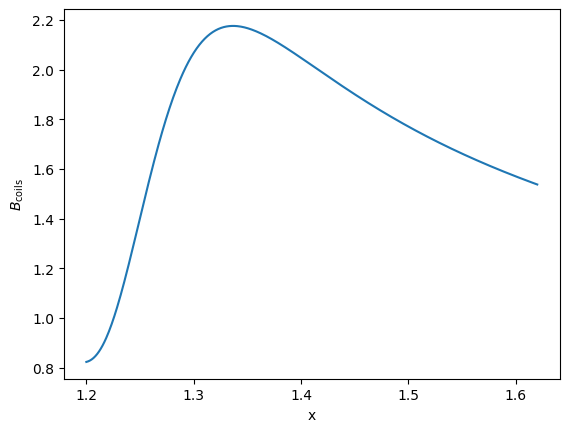
import matplotlib.pyplot as plt
ds_B = coil_set.eval_mod_B(eval_pos)
# plot the coil-field magnitude along a line
fig, ax = plt.subplots()
ax.plot(ds_B.pos.sel(xyz="x"), ds_B.mod_B)
ax.set(xlabel="x", ylabel=r"$B_{\text{coils}}$");
The same syntax holds for a single Coil
coil_set["coil_0"].eval_B(eval_pos)
<xarray.Dataset> Size: 24kB
Dimensions: (xyz: 3, points: 500)
Coordinates:
* xyz (xyz) <U1 12B 'x' 'y' 'z'
Dimensions without coordinates: points
Data variables:
B (xyz, points) float64 12kB 1.093 1.097 1.101 ... 0.03239 0.03215
pos (xyz, points) float64 12kB 1.2 1.201 1.202 1.203 ... 0.0 0.0 0.0Fieldline tracing in Cartesian coordinates#
fieldline tracing in \(x,y,z\) avoids issues for geometries beyond cylindrical coordinates (e.g. in G-Frame)
fieldline tracing core routine
trace_fieldlinestrace_fieldlineswrapsscipy.integrate.solve_ivpnecessary inputs for
trace_fieldlinesare the starting positions of the fieldlines, the coil-set and the time for how long to trace the fieldlinesprovide surface normals and surface points to specify planes on which intersections with the fieldlines are tracked \(\rightarrow\) Poincaré plots
The fieldline equations that are solved are
Where \(\mathbf{x}\) denotes the position vector.
In the example below we utilize the NCSX coilset to trace fieldlines.
Defining starting positions#
As an initial setup we define the starting positions for our fieldlines. For this NCSX case cylindrical coordinates are more convenient to use, hence we specify the starts first in \(R,Z,\phi\) and then translate those into x,y,z.
n_fieldlines = 2 # number of initialized fieldlines
# define starting positions for the fieldlines in R/Z/phi
R_start = np.linspace(1.5, 1.56, n_fieldlines)
Z_start = np.zeros_like(R_start)
phis_start = np.zeros_like(R_start)
# translate R/Z/Phi starts into xyz
starts = np.zeros([3, n_fieldlines])
starts[0, :] = R_start * np.cos(phis_start)
starts[1, :] = R_start * np.sin(phis_start)
starts[2, :] = Z_start
Terminating tracing early#
Sometimes it might be beneficial to terminate the fieldline tracing early, for example, when the fieldline leaves the relevant region. For such cases one can provide event routines to solve_ivp with the terminal attribute. In our case, we want to terminate the tracing if the fieldline crosses some \(R, Z\) limits. Below we show how such an event can be defined, for details see the solve_ivp documentation.
# limit the region where the fieldline is traced
trace_limits_R = [0.43600, 2.43600]
trace_limits_Z = [-1, 1]
# define a terminating event for the fieldline tracing
def terminal_event(t, xyz):
R = np.sqrt(xyz[0] ** 2 + xyz[1] ** 2)
if (trace_limits_R[0] <= R <= trace_limits_R[1]) and (
trace_limits_Z[0] <= xyz[2] <= trace_limits_Z[1]
):
return -1
else:
print(f"Terminate Fieldline: R={R:.2f}, Z={xyz[2]:.2f}")
return 0
terminal_event.terminal = True
Automatic event creation via planes#
To be able to plot Poincaré sections, we have to provide events to solve_ivp that occur when a fieldline crosses the relevant plane. In trace_fieldlines, such events can be automatically generated by providing surface normals (and optionally surface points). Here, we want to visualize \(\phi=const.\) cross-sections, thus we specify the corresponding surface normals.
n_planes = 4 # number of intersection planes for Poincaré plots
# define surface normals for of the intersection planes
phis = np.array([0, np.pi / 6, np.pi / 3, np.pi / 2])
surf_normals = [
np.array([-np.sin(phi), np.cos(phi), 0]) for phi in phis
]
Start the fieldline tracing#
parallelized over fieldlines \(\rightarrow\) set
n_jobs\(>1\)finer control via
solve_ivpkeyword arguments,atol,rtol,eventsetc.returns
xarray.Datatreecontaining the relevant data grouped for each fieldline
from gvec.coils import trace_fieldlines
tree = trace_fieldlines(
starts=starts, # initial positions for the fieldlines
coils=coil_set, # Object for evaluating the B-field
time=200, # time to trace fieldlines
surf_normals=surf_normals, # intersection planes
# surf_points = None # note that without surf_points the planes are expected to go through the origin
# solve_ivp specific keywords
events=[terminal_event],
atol=1e-5, # tune these tol. for more accurate results
rtol=1e-4,
)
INFO Tracing fieldlines using n_jobs=1
0%| | 0/2 [00:00<?, ?it/s]
50%|█████ | 1/2 [00:11<00:11, 11.84s/it]
100%|██████████| 2/2 [00:23<00:00, 11.95s/it]
100%|██████████| 2/2 [00:23<00:00, 11.93s/it]
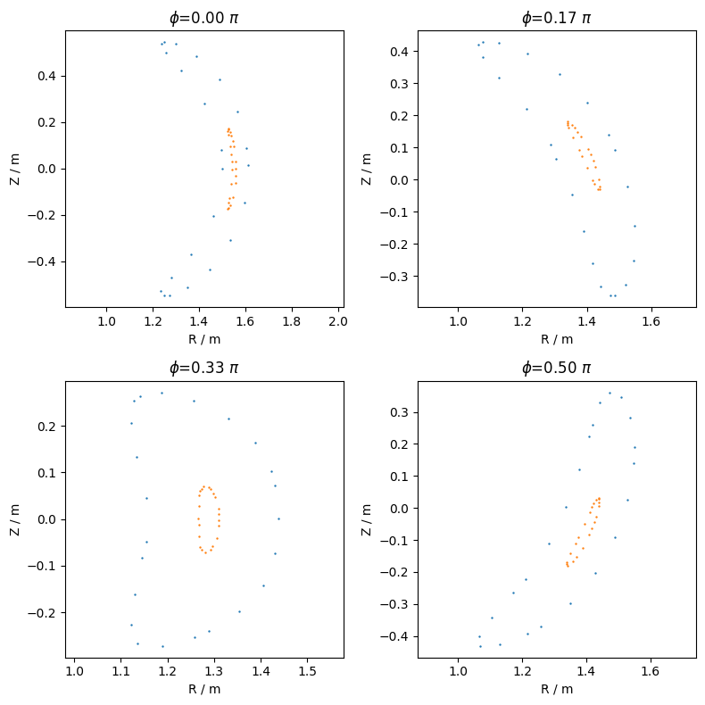
Poincaré plots#
To visualize the Poincaré cross-sections, we have to extract the intersection positions of each fieldline with the specified planes.
Intersection positions can be extracted for each fieldline via the event entry in the data set, numbered according to the order of the specified surface normals. Below we showcase a possible way to visualize the Poincaré sections using the returned data-tree.
fig, axs = plt.subplots(2, 2, figsize=(8, 8), tight_layout=True)
for fieldline in tree:
# select the relevant fieldline
ds = tree[fieldline]
try: # continue if the fieldline never intersected with any plane
for i, ax in enumerate(axs.flatten()):
# select intersection positions for the i-th plane
events = ds[
f"event_{i}"
] # corresponds to surface_normal[i]
# xyz --> RZphi
R = np.sqrt(
events.sel(xyz="x") ** 2 + events.sel(xyz="y") ** 2
)
ax.scatter(
R[
::2
], # select every other point to just get one Poincaré section
events.sel(xyz="z")[::2],
marker=".",
s=2,
)
except KeyError:
continue
# add some plot labels and titles
for ax, phi in zip(axs.flatten(), phis):
ax.set(
xlabel="R / m",
ylabel="Z / m",
title=f"$\\phi$={phi / np.pi:.2f} $\\pi$",
)
ax.axis("equal")
Visualizing the fieldlines in 3D#
With the data in the returned data-tree, we can also do some 3D visualizations to inspect the fieldlines and Poincaré sections with respect to the coils. Below is one example of how this could be achieved, again using the plotly package.
from plotly import graph_objects as go
# plot the coils
ax = coil_set.plot(
show=False,
line={"color": "black"},
showlegend=False,
)
ax["layout"]["scene"]["aspectmode"] = "data"
for fieldline in tree:
# plot the fieldlines
ds = tree[fieldline]
ax.add_trace(
go.Scatter3d(
x=ds.pos.sel(xyz="x"),
y=ds.pos.sel(xyz="y"),
z=ds.pos.sel(xyz="z"),
mode="lines",
opacity=0.2,
line={"color": "green"},
showlegend=False,
)
)
# starting positions
ax.add_trace(
go.Scatter3d(
x=starts[0, :],
y=starts[1, :],
z=starts[2, :],
mode="markers",
marker=dict(size=3, color="red"),
showlegend=False,
)
)
# plot the Poincaré sections in 3D
try:
for i in range(len(phis)):
ax.add_trace(
go.Scatter3d(
x=np.array(ds[f"event_{i}"].sel(xyz="x")),
y=np.array(ds[f"event_{i}"].sel(xyz="y")),
z=np.array(ds[f"event_{i}"].sel(xyz="z")),
mode="markers",
marker=dict(size=2, color="blue"),
showlegend=False,
)
)
except KeyError:
continue
ax.show();