G-Frame feature#
In this tutorial we want to give an overview of the G-Frame feature of GVEC.
The notebook covers the following steps:
Explain what the idea of the G-Frame is and its requirements
Construct a G-Frame from a simple curve and run GVEC
Rotate the G-Frame and rerun GVEC
Compare the G-Frame cross-sections of the rotated configuration with cross-sections in cylinder coordinates (\(R,Z\))
Construct a G-Frame from a knotted curve and run GVEC
Construct a G-Frame from a given surface and run in GVEC
Idea of the G-Frame#
In Stellarator research, the near-axis expansion (NAE) describes an equilibrium solution close to the axis. Depending on the order of the expansion, the validity of the equilibrium solution is extended further away from the magnetic axis.
A key to the NAE is the description of the coordinates: they are aligned with the magnetic axis, which is typically described by a Frenet-Serret frame. The coordinate frame is then described by a set of planes orthogonal to the axis, which are spanned by the normal and binormal of the local Frenet-Serret frame. In each of these planes the plasma shape can be described by two coordinates.
The magnetic axis follows the primary orientation of the plasma boundary. Therefore the cross-sections of the boundary surface become much less shaped when cutting it in planes perpendicular to the magnetic axis, instead of using cross-sections in \(R,Z\) (cylinder coordinates).
However, just using any closed curve to define a local Frenet-Serret frame may fail. There is an issue that the Frenet frame is not defined at points of zero curvature, and can abruptly flip its orientation when crossing those points. For planar curves this is not an issue, but it may be when the axis has a three dimensional shape with inflexion points — for instance, the magnetic axis of a stellarator optimised for quasi-isodynamicity has inflexion points.
In Hindenlang et al.(2025) we introduced the ‘G-Frame’, which serves as an interface to define the coordinate frame in GVEC. It consists of a closed curve \(\mathbf{X}_0(\zeta)\), with curve parameter \(\zeta \in [0,2\pi]\), that describes the origin of the planes. The planes are spanned by two additional unit vectors \(\mathbf{N}(\zeta)\) and \(\mathbf{B}(\zeta)\) and thus define a map between the two coordinates \(X^1(\rho,\theta,\zeta)\), \(X^2(\rho,\theta,\zeta)\) in the \(\mathbf{N},\mathbf{B}\) planes and the cartesian coordinates \(\mathbf{x}\). The map is denoted \(h\) and hmap in the code,
Requirements for the G-Frame#
Note that the name ‘G-Frame’ does not refer to a particular construction from a curve (like “Frenet-Serret”, or “Bishop”, or “Minimal-Rotating”), but rather to a ‘general’ definition of a coordinate frame. It can be seen as a set of smoothly varying planes along the origin curve. A G-Frame has to fulfill the following properties:
The origin curve \(\mathbf{X}_0(\zeta)\) must be closed.
A valid plane must be spanned by the vectors \(\mathbf{B}(\zeta)\) and \(\mathbf{N}(\zeta)\), meaning \((\mathbf{N}\times \mathbf{B})\cdot \mathbf{X}_0^\prime > 0\) for all \(\zeta\).
Even though not strictly necessary, it is recommended to use unit vectors and orthogonality in the plane, i.e. \(|\mathbf{N}\times \mathbf{B}|=1\).
All vectors must be continuous and smoothly varying over \(\zeta\). Internally, they will be represented by Fourier series.
The origin curve \(\mathbf{X}_0\) and two vectors \(\mathbf{N}\) and \(\mathbf{B}\) are given in cartesian coordinates, sampled along the curve parameter over the full torus
\[\begin{align*} \zeta_k = \frac{2\pi k}{N_\zeta N_{\rm FP}}, k=0,\dots,N_\zeta N_{\rm FP}-1 \end{align*} \]where \(N_\zeta\) is the number of points per field period, and \(N_{FP}\) is the number of field periods. This definition allows for explicitly checking the field-periodicity of the data \(\mathbf{X}_0(\zeta_k)\), \(\mathbf{N}(\zeta_k)\) and \(\mathbf{B}(\zeta_k)\).
More details on the G-Frame are found in our publication Hindenlang et al.(2025).
# set the number of OpenMP threads before importing gvec
import os
os.environ["OMP_NUM_THREADS"] = "2"
import numpy as np
import matplotlib.pyplot as plt
import gvec
Constructing a G-Frame from a simple curve#
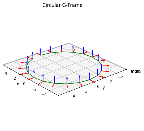
Now lets simply construct a G-Frame from a circular curve, and write it to a netcdf file that GVEC can read, using gvec.gframe.write_Gframe_ncfile(🌐):
# number of field periods
nfp = 1
# number of points along the axis, per field period
nzeta = 20
zetafull = np.linspace(0, 2 * np.pi, nzeta * nfp, endpoint=False)
xyz = np.zeros((3, zetafull.shape[0]))
Nxyz = np.zeros_like(xyz)
Bxyz = np.zeros_like(xyz)
# a circular curve with radius 5, in clockwise direction seen from above
xyz[0, :] = 5 * np.cos(zetafull)
xyz[1, :] = 5 * np.sin(-zetafull)
# First vector N is outward pointing
Nxyz[0, :] = np.cos(zetafull)
Nxyz[1, :] = np.sin(-zetafull)
# Second vector B points in Z direction
Bxyz[2, :] = 1.0
# write the G-Frame to a netcdf file, using a dictionary
dict_gframe = {
"nfp": nfp,
"axis": {
"nzeta": nzeta,
"zetafull": zetafull,
"xyz": xyz,
"Nxyz": Nxyz,
"Bxyz": Bxyz,
},
}
gvec.gframe.write_Gframe_ncfile("circular-gframe.nc", dict_gframe)
lets have a look at the data of the resulting G-Frame:
def plot_gframe(dict_in, title="G-Frame", length=1):
fig = plt.figure(figsize=(5, 5), tight_layout=True)
ax = fig.add_subplot(111, projection="3d")
x, y, z = dict_in["axis"]["xyz"]
Nx, Ny, Nz = dict_in["axis"]["Nxyz"]
Bx, By, Bz = dict_in["axis"]["Bxyz"]
ax.plot3D(x, y, z, color="green")
ax.quiver3D(x, y, z, Nx, Ny, Nz, color="red", length=length)
ax.quiver3D(x, y, z, Bx, By, Bz, color="blue", length=length)
ax.set(aspect="equal")
ax.set_xlabel("x")
ax.set_ylabel("y")
ax.set_zlabel("z")
ax.set_title(title)
ax.view_init(25, 140, 0)
return fig, ax
fig, ax = plot_gframe(dict_gframe, title="Circular G-Frame")
Using the G-Frame in a GVEC run#
We now try to rerun the tokamak example from tutorial Elliptic Tokamak(🌐), with the same parameters, but using the G-Frame we just constructed.
Note that since the Fourier coefficients of the boundary in \(X^1,X^2\) are now given in terms of the G-Frame, the origin \((X^1,X^2)=(0,0)\) is represented by the origin curve \(\mathbf{X}_0(\zeta)\), which has a radius of \(5\), whereas for the cylinder coordinates (which_hmap=1), the origin would be at \(\mathbf{x}=(0,0,0)\).
Thus we set the parameters which_hmap and hmap_ncfile for the G-Frame, and set the Fourier coefficient X1_b_cos[0,0] to 0 instead of 5. All other parameters remain unchanged.
params = {"ProjectName": "GVEC_elliptok_gframe"}
# set hmap to the G-Frame, provided as a netcdf file
params["which_hmap"] = 21
params["hmap_ncfile"] = (
"../circular-gframe.nc" # path relative to run directory
)
# number of field periods
params["nfp"] = 1
# boundary modes. Note that G-Frame changes origin, so (0,0) is now =0.0 !
params["X1_b_cos"] = {
(0, 0): 0.0,
(1, 0): 0.9,
}
params["X2_b_sin"] = {(1, 0): 1.1}
# append remaining parameters, based on tokamak case
params |= {
# profile definitions for iota and pressure -------------------
# total toriodal flux (scales magnetic field stength)
"PhiEdge": 1.0,
"iota": {
"type": "polynomial",
"coefs": [0.625, 0.35],
},
"pres": {
"type": "polynomial",
"coefs": [1.0, -1.0],
"scale": 1000.0,
},
# radial resolution parameters ---------------------------------
# number of radial B-spline elements
"sgrid_nElems": 2,
# degree of B-splines for X1 and X2
"X1X2_deg": 5,
# degree of B-splines for LA
"LA_deg": 5,
# Minimizer parameters -----------------------------------------
# maximum number of iterations
"totalIter": 10000,
# abort tolerance on sqrt(|forces|^2) in the energy minimization
"minimize_tol": 1e-6,
# optional parameters ------------------------------------------
"logIter": 100, # log interval for diagnostics
}
# write parameters to file
gvec.util.write_parameters(params, "elliptok_gframe_parameters.toml")
and now lets run the GVEC code
runpath = "run_elliptok_gframe"
run = gvec.run(
params, runpath=runpath
) # overwrites runpath or creates a new one
GVEC - completed 0/2 stages: |>|.|
GVEC - completed 1/2 stages: |=|>|
GVEC finished after 2.0 seconds using 2550 iterations (totalIter = 10000) with |force| = 9.97e-07 (minimize_tol = 1.00e-06)
and generate the same plot as we did in the elliptic tokamak tutorial
def visualize_cross_section(state):
rho = np.linspace(0, 1, 20) # radial visualization points
theta = np.linspace(
0, 2 * np.pi, 50
) # poloidal visualization points
ev = state.evaluate(
"X1",
"X2",
"LA",
"iota",
"p",
rho=rho,
theta=theta,
zeta=[0.0],
)
fig, ax = plt.subplots(1, 1, figsize=(8, 5))
R = ev.X1[:, :, 0]
Z = ev.X2[:, :, 0]
R_axis = R[0, 0].item()
Z_axis = Z[0, 0].item()
rho_vis = R * 0 + ev.rho
thetastar_vis = ev.LA[:, :, 0] + ev.theta
p_vis = R * 0 + ev.p
rho_levels_vis = np.linspace(0, 1 - 1e-10, 11)
theta_levels_vis = np.linspace(0, 2 * np.pi, 16, endpoint=False)
c = ax.contourf(R, Z, p_vis, alpha=0.75)
fig.colorbar(c, ax=ax, label="pressure")
ax.contour(R, Z, rho_vis, rho_levels_vis, colors="black")
ax.contour(R, Z, thetastar_vis, theta_levels_vis, colors="red")
ax.set(
xlabel="$X^1$",
ylabel="$X^2$",
title=f"equilibrium solution, circular G-Frame,cross-section $\zeta=0$, \n position of magnetic axis $(X^1,X^2)$=({R_axis:.5f},{Z_axis:.5f})",
aspect="equal",
xlim=[1.1 * np.amin(R), 1.1 * np.amax(R)],
ylim=[1.1 * np.amin(Z), 1.1 * np.amax(Z)],
)
ax.legend(
handles=[
plt.Line2D(
[0], [0], color="black", label="$\\rho=$const."
),
plt.Line2D(
[0], [0], color="red", label="$\\vartheta^*=$const"
),
]
)
return fig
state = gvec.find_state("run_elliptok_gframe")
fig = visualize_cross_section(state)
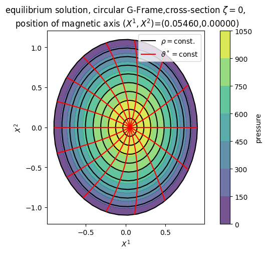
The resulting cross-section is exactly the same. Here, the solution of \(X^1,X^2\) in the \(\zeta=0\) plane of the G-Frame is shown. Notice the shift of the magnetic axis with respect to the new origin \((X^1,X^2)=(0,0)\).
Rotate the G-Frame#
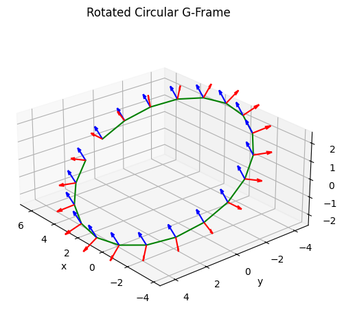
Lets now rotate the previous G-Frame by \(\pi/6\) around the \(x\)-axis and also shift it along the \(x\)-axis:
xyz = dict_gframe["axis"]["xyz"]
Nxyz = dict_gframe["axis"]["Nxyz"]
Bxyz = dict_gframe["axis"]["Bxyz"]
rotangle = np.pi / 6
# rotation matrix around x axis:
rotmat = np.array(
[
[1, 0, 0],
[0, np.cos(rotangle), np.sin(rotangle)],
[0, -np.sin(rotangle), np.cos(rotangle)],
]
)
xyz_rotated = rotmat @ xyz
Nxyz_rotated = rotmat @ (xyz + Nxyz) - xyz_rotated
Bxyz_rotated = rotmat @ (xyz + Bxyz) - xyz_rotated
xyz_rotated[0, :] += 1.25
dict_gframe_rotated = {
"nfp": nfp,
"axis": {"nzeta": nzeta, "zetafull": zetafull},
}
dict_gframe_rotated["axis"]["xyz"] = xyz_rotated
dict_gframe_rotated["axis"]["Nxyz"] = Nxyz_rotated
dict_gframe_rotated["axis"]["Bxyz"] = Bxyz_rotated
gvec.gframe.write_Gframe_ncfile(
"rotated-circular-gframe.nc", dict_gframe_rotated
)
fig, ax = plot_gframe(
dict_gframe_rotated, title="Rotated Circular G-Frame"
)
We keep the same parameters but exchange the G-Frame file, and rerun GVEC:
params_rotated = params.copy()
params_rotated["ProjectName"] = "GVEC_elliptok_gframe_rotated"
# path relative to run directory
params_rotated["hmap_ncfile"] = "../rotated-circular-gframe.nc"
runpath = "run_elliptok_gframe_rotated"
run = gvec.run(params_rotated, runpath=runpath)
GVEC - completed 0/2 stages: |>|.|
GVEC - completed 1/2 stages: |=|>|
GVEC finished after 2.0 seconds using 2550 iterations (totalIter = 10000) with |force| = 9.97e-07 (minimize_tol = 1.00e-06)
# load the state from the runpath and visualize
state = gvec.find_state("run_elliptok_gframe_rotated")
fig = visualize_cross_section(state)
Obviously, since only the orientation of the G-Frame has changed, but the boundary modes remained the same, we get the exact same cross-section of the solution in \(X^1,X^2\) at \(\zeta=0\).
Note that this is now the cross-section of the rotated G-Frame, rather than a cross-section in cylinder coordinates.
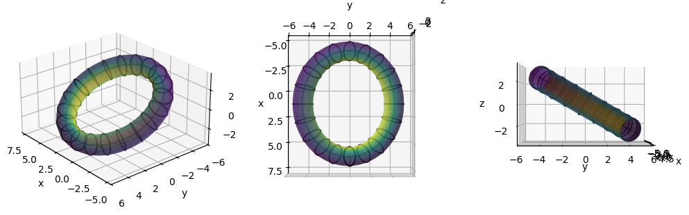
In order to see that the solution is actually rotated, we visualize now the magnetic axis and the boundary in 3D, and also show mod_B on the boundary:
# function to visualize in 3D
def boundary_views_3D(xyz_bnd, xyz_axis=None, scalar=None):
fig = plt.figure(figsize=(10, 8), tight_layout=True)
nzeta = xyz_bnd.shape[0]
axs = [None, None, None]
for i in range(3):
ax = fig.add_subplot(1, 3, i + 1, projection="3d", alpha=0.9)
axs[i] = ax
if scalar is not None:
norm_scalar = (scalar - np.amin(scalar)) / (
np.amax(scalar) - np.amin(scalar)
)
cmap = plt.get_cmap("viridis")
fc = cmap(norm_scalar)
else:
fc = None
ax.plot_surface(
xyz_bnd[:, :, 0],
xyz_bnd[:, :, 1],
xyz_bnd[:, :, 2],
facecolors=fc,
edgecolor=None,
alpha=0.6,
)
if xyz_axis is not None:
ax.plot(
xyz_axis[:, 0],
xyz_axis[:, 1],
xyz_axis[:, 2],
color="g",
alpha=0.6,
)
for iz in range(0, nzeta, nzeta // 20):
ax.plot(
xyz_bnd[iz, :, 0],
xyz_bnd[iz, :, 1],
xyz_bnd[iz, :, 2],
color="k",
alpha=0.7,
)
ax.set(aspect="equal")
ax.set_xlabel("x")
ax.set_ylabel("y")
ax.set_zlabel("z")
axs[0].view_init(25, 140, 0)
axs[1].view_init(90, 0, 0)
axs[2].view_init(0, 0, 0)
return fig, axs
# evaluate the boundary and axis geometry
zeta_visu = np.linspace(0, 2 * np.pi, 81)
theta_visu = np.linspace(0, 2 * np.pi, 41)
ev_bnd = (
state.evaluate(
"pos", "mod_B", rho=1.0, theta=theta_visu, zeta=zeta_visu
)
.sel(rho=1.0)
.transpose("tor", "pol", "xyz")
)
xyz_bnd = np.asarray(ev_bnd.pos)
ev_axis = state.evaluate("pos", rho=0.0, theta=0.0, zeta=zeta_visu)
xyz_axis = np.asarray(
ev_axis.pos.sel(rho=0.0).sel(theta=0.0).transpose("tor", "xyz")
)
# visualize
fig, axs = boundary_views_3D(
xyz_bnd, xyz_axis=xyz_axis, scalar=np.asarray(ev_bnd.mod_B)
)
Add boundary surface to G-Frame file#
The netcdf file that contains the G-Frame (axis group) can additionally contain the \(X^1(\vartheta,\zeta),X^2(\vartheta,\zeta)\) positions of the boundary in one field period (in a boundary group).
We simply extend the dictionary with the boundary positions, and write it to file again:
# sample boundary with a minimal resolution
ntheta_bnd = 5
nzeta_bnd = 3
theta_bnd = np.linspace(0, 2 * np.pi, ntheta_bnd, endpoint=False)
zeta_bnd = np.linspace(0, 2 * np.pi / nfp, nzeta_bnd, endpoint=False)
ev_bnd = state.evaluate(
"X1", "X2", rho=1.0, theta=theta_bnd, zeta=zeta_bnd
).sel(rho=1.0)
# combine "axis" from dict_gframe_rotated and "boundary"
dict_all_rotated = dict_gframe_rotated.copy()
dict_all_rotated["boundary"] = {
"nzeta": nzeta_bnd,
"zeta": zeta_bnd,
"n_max": 0,
"ntheta": ntheta_bnd,
"theta": theta_bnd,
"m_max": 1,
"X1": np.asarray(ev_bnd.X1.transpose("pol", "tor")),
"X2": np.asarray(ev_bnd.X2.transpose("pol", "tor")),
"lasym": False,
}
# write everything to a netcdf file
gvec.gframe.write_Gframe_ncfile(
"rotated-circular-gframe-and-boundary.nc", dict_all_rotated
)
Compare cross-sections, G-Frame vs cylinder coordinates#
We can generate a boundary surface object from the last dictionary, using
gvec.gframe.to_surface(🌐), or alternatively read it from the previously written G-frame file.
Then we cut it in cylinder coordinates to compare the cross-sections, using
gvec.gframe.to_RZ(🌐).
# read from previously written file (not necessary here)
# dict_all_rotated = gvec.gframe.read_Gframe_ncfile("rotated-circular-gframe-and-boundary.nc")
# extract the boundary surface
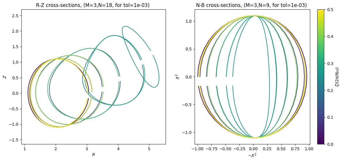
dict_surf = gvec.gframe.to_surface(dict_all_rotated)
# cut the boundary surface to RZ cross sections
dict_RZ = gvec.gframe.to_RZ(dict_surf["xyz"], dict_surf["nfp"])
# plot comparison
fig = gvec.gframe.plot_cross_section_comparison(
dict_surf, dict_RZ, step=4
)
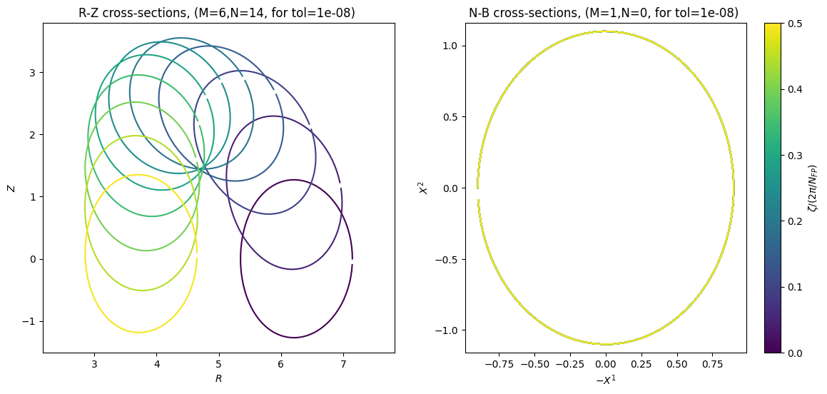
The visualization reveals that in order to represent the same tilted surface in cylinder coordinates (up to a tolerance of 1e-8), we would need maximum Fourier mode numbers of \(M=6,N=14\).
This comparison is very useful to see the effect of the G-Frame. It can be easily applied to other G-Frame files, i.e. those generated from the QUASR database.
The details on how to generate it from a QUASR case are described in GVEC-QUASR interface(🌐).
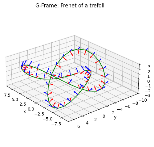
Generate the G-Frame from a Frenet frame#
If the origin curve has non-zero curvature everywhere, we can use the Frenet-Serret formulas for computing a G-Frame.
We show the construction with an origin curve from the trefoil knot, which has only non-zero curvature.
def trefoil(t):
x = np.sin(t) + 2 * np.sin(2 * t)
y = np.cos(t) - 2 * np.cos(2 * t)
z = -np.sin(3 * t)
X0 = np.stack((x, y, z), axis=0)
xp = np.cos(t) + 4 * np.cos(2 * t)
yp = -np.sin(t) + 4 * np.sin(2 * t)
zp = -3 * np.cos(3 * t)
X0p = np.stack((xp, yp, zp), axis=0)
xpp = -np.sin(t) - 8 * np.sin(2 * t)
ypp = -np.cos(t) + 8 * np.cos(2 * t)
zpp = 9 * np.sin(3 * t)
X0pp = np.stack((xpp, ypp, zpp), axis=0)
xppp = -np.cos(t) - 16 * np.cos(2 * t)
yppp = np.sin(t) - 16 * np.sin(2 * t)
zppp = 27 * np.cos(3 * t)
X0ppp = np.stack((xppp, yppp, zppp), axis=0)
scale = 3
return scale * X0, scale * X0p, scale * X0pp, scale * X0ppp
def frenet(X0p, X0pp, X0ppp):
lp = np.sqrt(np.sum(X0p**2, axis=0))
B = np.cross(X0p, X0pp, axis=0)
Bnorm = np.sqrt(np.sum(B**2, axis=0))
kappa = Bnorm / (lp**3)
tau = np.sum(B * X0ppp, axis=0) / Bnorm**2
B = B / Bnorm[None, :]
T = X0p / lp[None, :]
N = np.cross(B, T, axis=0)
return T, N, B, lp, kappa, tau
nz = 15
zf = np.linspace(0, 2 * np.pi, 3 * nz, endpoint=False)
X0, X0p, X0pp, X0ppp = trefoil(zf)
T, N, B, lp, kappa, tau = frenet(X0p, X0pp, X0ppp)
dict_gframe_trefoil = {
"nfp": 3,
"axis": {"nzeta": nz, "zetafull": zf},
}
dict_gframe_trefoil["axis"]["xyz"] = X0
dict_gframe_trefoil["axis"]["Nxyz"] = N
dict_gframe_trefoil["axis"]["Bxyz"] = B
fig, ax = plot_gframe(
dict_gframe_trefoil, title="G-Frame: Frenet of a trefoil"
)
gvec.gframe.write_Gframe_ncfile(
"trefoil-gframe.nc", dict_gframe_trefoil
)
Run in GVEC#
params_trefoil = params.copy()
params_trefoil["ProjectName"] = "GVEC_elliptok_gframe_trefoil"
# path relative to run directory
params_trefoil["hmap_ncfile"] = "../trefoil-gframe.nc"
runpath = "run_elliptok_gframe_trefoil"
run = gvec.run(params_trefoil, runpath=runpath)
GVEC - completed 0/2 stages: |>|.|
GVEC - completed 1/2 stages: |=|>|
GVEC finished after 3.7 seconds using 7058 iterations (totalIter = 10000) with |force| = 9.99e-07 (minimize_tol = 1.00e-06)
and visualize in 3D:
state = gvec.find_state("run_elliptok_gframe_trefoil")
ev_bnd = (
state.evaluate(
"pos", "mod_B", rho=1.0, theta=theta_visu, zeta=zeta_visu
)
.sel(rho=1.0)
.transpose("tor", "pol", "xyz")
)
xyz_bnd = np.asarray(ev_bnd.pos)
ev_axis = state.evaluate("pos", rho=0.0, theta=0.0, zeta=zeta_visu)
xyz_axis = (
ev_axis.pos.sel(rho=0.0).sel(theta=0.0).transpose("tor", "xyz")
)
fig, axs = boundary_views_3D(
xyz_bnd, xyz_axis=xyz_axis, scalar=np.asarray(ev_bnd.mod_B)
)
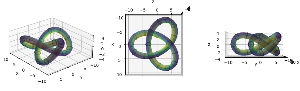
or use the inbuild 3D plotting function state.plot_3d_surface(🌐) (plotly), as described in the tutorial Plotting(🌐).
fig = state.plot_3d_surface(
period="full",
zeta_contours=8,
surface_kwargs=dict(opacity=0.5),
)
fig.show();
Generate the G-Frame from a surface#
Another way of constructing a G-Frame is from a given surface, for example from the QUASR database as described in Hindenlang et. al. (2025). The algorithm aligns the planes of the G-Frame with contours of constant \(\zeta\) on the input surface. We found that starting from a surface parameterized in Boozer angles makes the G-Frame follow nicely the shape of the boundary and can find cross-sections that are close to perpendicular to the magnetic axis.
Another advantage when starting from a surface is that one can use it as the boundary flux surface of the equilibrium.
Input surface#
The surface must be non-self-intersecting, and the normal has to be oriented outwards, such that the enclosed volume is positive.
The input surface is given as an array of 3D cartesian points xyz[0:nzeta*nfp,0:ntheta,0:2], with the number of points in poloidal direction ntheta and the number of points in toroidal direction nzeta*nfp, making the discrete points exactly field-periodic. For example, having a function eval_surface to evaluate a point on the surface \(\mathbf{x}(\theta,\zeta)\), one can generate the data as
theta=np.linspace(0,2*np.pi,ntheta,endpoint=False)
zeta=np.linspace(0,2*np.pi,nzeta*nfp,endpoint=False)
xyz=np.zeros((nzeta*nfp,ntheta,3))
for j in range(nzeta*nfp):
for i in range(ntheta):
xyz[j,i,:] = eval_surface(theta[i],zeta[j])
Note that since the G-Frame cross-sections will be aligned to \(\zeta\) contours, if \(\zeta\) is the geometric toroidal angle in cylinder coordinates, the cross-sections in the G-Frame will remain \(R,Z\) cross-sections.
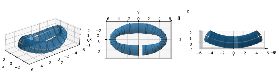
Here, for simplicity, we start from the axisymmetric surface data from the first case above, and apply a non-linear deformation to make it non-axisymmetric. Note that this also deforms the \(\zeta=\text{constant}\) contours on the surface.
state = gvec.find_state("run_elliptok_gframe")
ev = state.evaluate("pos", rho=1.0, theta=40, zeta=40).sel(rho=1.0)
xyz_bnd = np.asarray(ev.pos.transpose("tor", "pol", "xyz"))
def deform_ring(x, y, z):
"""
deform a circular ring (in xy-plane) to an elliptic ring via a conformal map
"""
r = np.sqrt(x**2 + y**2)
t = np.arctan2(y, x)
w = np.sin(t + 1j * (r / 5 - 0.6))
return np.imag(w) * 5, np.real(w) * 5, z
def deform_yz(x, y, z, z_origin=10):
"""deform in yz-plane, z=const lines to circles with center y=0,z=z_origin"""
r = z_origin - z
t = np.arctan(np.amax(y) / z_origin) * y / np.amax(y)
znew = z_origin - r * np.cos(t)
ynew = r * np.sin(t)
return x, ynew, znew
x, y, z = np.unstack(xyz_bnd, axis=2)
x, y, z = deform_ring(x, y, z)
x, y, z = deform_yz(x, y, z)
xyz_bnd = np.stack((x, y, z), axis=2)
fig, axs = boundary_views_3D(xyz_bnd)

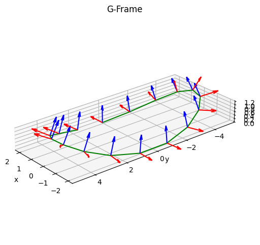
Construct the G-Frame#
We have now a surface in 3D and can generate the G-Frame from it with the function
gvec.gframe.construct_gframe_from_surface(🌐).
The output is a dictionary for the G-Frame and its boundary, as well as a list of GVEC parameters. The function also writes the parameters and the dictionary to file.
Two important parameters are used here:
tolerance_output: Maximum allowed distance between the original input surface and the surface represented with a finite number of Fourier modes in \(X^1,X^2\) in the G-Frame. The larger the tolerance, the lower the number of Fourier modes needed.cutoff_gframe: Maximal number of Fourier modes per field period to represent the G-Frame. Default =-1 is no cutoff, using the number of toroidal modes of the input surface. The lower the number of modes in the G-Frame, the cheaper becomes its evaluation in the GVEC equilibrium solve. However, depending on the output tolerance, a low cutoff can increase again the number of Fourier modes in \(X^1,X^2\).
# print the INFO level of the gframe construction algorithm
import logging
logger = logging.getLogger(__name__)
logger.setLevel(logging.INFO)
# construct the gframe from surface
params_deformed, dict_gframe_deformed = (
gvec.gframe.construct_gframe_from_surface(
xyz_bnd,
nfp=1,
name="deformed_surface",
tolerance_output=1e-3,
cutoff_gframe=8,
logger=logger,
)
)
INFO . check field periodicity
INFO . analyze input surface
INFO - input surface is NOT stellarator-symmetric (symmetric if xhat~cos,yhat~sin,zhat~sin):
INFO max|xhat_c|=3.4000838132467344, max|xhat_s|=0.2618896229919736,
INFO max|yhat_c|=0.1322841936543171, max|yhat_s|=3.4495427502271903,
INFO max|zhat_c|=0.5993573114044296, max|zhat_s|=1.0346632568068683.
INFO . Constructing the G-Frame
INFO - surface orientation right-handed, positive volume = 6.006e+01
INFO - linking number of the surface = -0 (number of poloidal windings around its center)
INFO - filter surface for G-frame construction with cutoff 8
INFO - G-frame linking number = -0, twist = -0.000, writhe = (Lk-Tw)= 0.000
INFO . Cutting the surface
INFO . Finding minimal modes for X^1,X^2, (M=20, N=20), with tolerance 1.0e-03
INFO Found minimal (M=3, N=9) for (X^1,X^2)
INFO - with maximum distance in the poloidal plane: 3.0e-03
INFO . output X^1,X^2 coordinates are NOT stellarator-symmetric:
INFO max|X1_c|=0.6972420804871782, max|X1_s|=0.006874604014943559,
INFO max|X2_c|=0.0014420742495563719, max|X2_s|=1.1000039017506171.
INFO . Exporting h-map & boundary
INFO . Writing files: deformed_surface-Gframe.nc , deformed_surface-parameters.yaml
INFO Done
and now we visualize the G-Frame and boundary that were generated:
fig, ax = plot_gframe(dict_gframe_deformed)
dict_surf_deformed = gvec.gframe.to_surface(
dict_gframe_deformed, nzeta=40, ntheta=40, tolerance=1e-3
)
fig, axs = boundary_views_3D(dict_surf_deformed["xyz"])
It is also possible to visualize the constructed G-Frame externally, for example in paraview, using gvec.vtk.gframe_to_vtk(🌐) to write several .vts files, providing the G-Frame netcdf file, and additional visualization parameters.
gvec.vtk.gframe_to_vtk(
"deformed_surface-Gframe.nc",
theta_visu=np.linspace(0, 2 * np.pi, 41),
zeta_visu=np.linspace(0, 2 * np.pi, 201),
quiet=False,
)
File output to /home/docs/checkouts/readthedocs.org/user_builds/gvec/checkouts/develop/docs/tutorials/notebooks/visu_axis.vts
Vector output variables: ['pos', 'N', 'B']
File output to /home/docs/checkouts/readthedocs.org/user_builds/gvec/checkouts/develop/docs/tutorials/notebooks/visu_boundary.vts
Scalar output variables: ['X1', 'X2']
Vector output variables: ['pos']
Cross-sections comparison#
We can again compare the cross-sections of the configuration in the G-Frame to cross-sections in cylinder coordinates, choosing the same matching tolerance to the original surface of 1e-3:
dict_RZ = gvec.gframe.to_RZ(
dict_surf_deformed["xyz"],
nfp,
nzeta=40,
ntheta=40,
tolerance=1e-3,
)
# plot comparison
fig = gvec.gframe.plot_cross_section_comparison(
dict_surf_deformed, dict_RZ, step=2
)
Run in GVEC#
Let’s first have a look at the predefined parameters from the construction of the G-Frame. All GVEC parameters are documented here(🌐).
The pressure is set to zero, as well as the toroidal current (see tutorial Prescribe a current profile(🌐) for more details). Also the maximum mode numbers and stellarator symmetry settings are automatically set from the G-Frame construction.
The boundary surface data from the G-Frame file is used instead of specifying boundary modes, see getBoundaryFromFile and boundary_filename parameters.
for key in params_deformed.keys():
print(f"{key:20}: {params_deformed[key]}")
ProjectName : deformed_surface
which_hmap : 21
hmap_ncfile : deformed_surface-Gframe.nc
X1X2_deg : 5
LA_deg : 5
sgrid : {'grid_type': 0, 'nElems': 5}
X1_mn_max : (3, 9)
X2_mn_max : (3, 9)
LA_mn_max : (3, 9)
X1_sin_cos : _sincos_
X2_sin_cos : _sincos_
LA_sin_cos : _sincos_
minimize_tol : 1e-07
totalIter : 100000
logIter : 100
pres : {'type': 'polynomial', 'coefs': [0.0]}
I_tor : {'type': 'polynomial', 'coefs': [0.0]}
picard_current : auto
init_average_axis : True
getBoundaryFromFile : 1
boundary_filename : deformed_surface-Gframe.nc
We adapt some of the parameters (path and minimizer tolerance) and run GVEC:
# change path to the netcdf file because the GVEC run is in a sub-directory
params_deformed["hmap_ncfile"] = "../deformed_surface-Gframe.nc"
params_deformed["boundary_filename"] = "../deformed_surface-Gframe.nc"
# increase tolerance so that the run is faster
params_deformed["minimize_tol"] = 1e-3
runpath = "run_deformed_gframe"
run = gvec.run(params_deformed, runpath=runpath)
GVEC - completed 0/3 stages, restarts in current stage - 0: |>|.|.|
GVEC - completed 1/3 stages, restarts in current stage - 0: |=|>|.|
GVEC - completed 2/3 stages, restarts in current stage - 0: |=|=|>|
GVEC finished after 6.7 seconds using 164 iterations (totalIter = 100000) with |force| = 9.72e-04 (minimize_tol = 1.00e-03)
and rms Δiota = 2.47e-14(iota_tol=1.00e-03)
and visualize cross-sections of the solution and the boundary:
state = gvec.find_state("run_deformed_gframe")
ev = state.evaluate(
"mod_B",
rho=20,
theta=np.linspace(0, 2 * np.pi, 31),
zeta=np.linspace(0, np.pi, 9),
)
# === Cross-sections === #
fig, axs = plt.subplots(
3, 3, figsize=(10, 8), sharex=True, sharey=True
)
vmin = np.amin(ev.mod_B)
vmax = np.amax(ev.mod_B)
r_levels = np.linspace(0, 1 - 1e-10, 5)
t_levels = np.linspace(0, 2 * np.pi, 9)
for ax, zeta_pos in zip(axs.flat, ev.zeta[:]):
# select zeta-plane from dataset
ev_z = ev.sel(zeta=zeta_pos, method="nearest")
c = ax.contourf(
ev_z.X1, ev_z.X2, ev_z.mod_B, vmin=vmin, vmax=vmax
)
ax.contour(
ev_z.X1,
ev_z.X2,
0 * ev_z.X1 + ev_z.rho,
r_levels,
colors="white",
alpha=0.7,
)
ax.contour(
ev_z.X1,
ev_z.X2,
0 * ev_z.X1 + ev_z.theta,
t_levels,
colors="white",
alpha=0.7,
)
ax.set(
aspect="equal",
title=f"$\\zeta/2\\pi = {zeta_pos / (2 * np.pi):.3f}$",
)
for ax in axs[-1, :]:
ax.set_xlabel(f"${ev.X1.attrs['symbol']}$")
for ax in axs[:, 0]:
ax.set_ylabel(f"${ev.X2.attrs['symbol']}$")
fig.colorbar(c, ax=axs, shrink=0.5, label="|B|")
ev_bnd = (
state.evaluate(
"pos", "mod_B", rho=1.0, theta=theta_visu, zeta=zeta_visu
)
.sel(rho=1.0)
.transpose("tor", "pol", "xyz")
)
xyz_bnd = np.asarray(ev_bnd.pos)
ev_axis = state.evaluate("pos", rho=0.0, theta=0.0, zeta=zeta_visu)
xyz_axis = (
ev_axis.pos.sel(rho=0.0).sel(theta=0.0).transpose("tor", "xyz")
)
fig, axs = boundary_views_3D(
xyz_bnd, xyz_axis=xyz_axis, scalar=np.asarray(ev_bnd.mod_B)
)
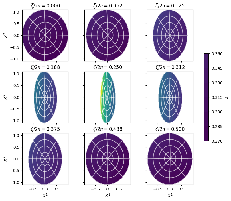
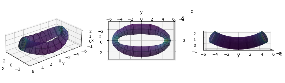
fig = state.plot_3d_surface(
period="full",
zeta_contours=15,
surface_kwargs=dict(opacity=0.5),
)
fig.show();