Prescribe a current profile#
Alternatively to fixing the \(\iota(s)\) profile, one can also fix the total toroidal current \(I_{\text{tor}}(s)\) when solving for an equilibrium. This notebook showcases how to do so in GVEC.
We start with the necessary imports and set the number of threads to use:
# set the number of OMP threads for gvec (needs to be before import of gvec)
import os

os.environ["OMP_NUM_THREADS"] = "2"
import gvec
In this tutorial, we load the parameters from the .toml file written in the tutorial Elliptic Stellarator(🌐)
params = gvec.util.read_parameters("ellipstell_parameters.toml")
New parameters#
Running GVEC with a prescribed \(I_{\text{tor}}(s)\) slightly changes the underlying algorithm. However, the basic syntax in terms of the parameters is almost the same as in the fixed \(\iota\) case.
The basic steps we need are:
prescribe \(I_{\text{tor}}(s)\) profile via
I_tor, with the same syntax to the one used foriotaandpresprofiles.set the new parameter
picard_currentoptionally provide an initial guess for \(\iota\)
For our stellarator example we choose to set I_tor to zero and utilize the automatic setup for picard_current by setting picard_current="auto".
Note that prescribing a toroidal current profile will always treat iota as an initial guess!
# toroidal current profile (=0)
params["I_tor"] = {
    "type": "polynomial",
    "coefs": [0.0],
}
# initial guess for iota (=0)
params["iota"] = {"type": "polynomial", "coefs": [0.0]}

params["picard_current"] = "auto"
params["minimize_tol"] = 1.0e-5
params["totalIter"] = 100000
Running GVEC with prescribed toroidal current#
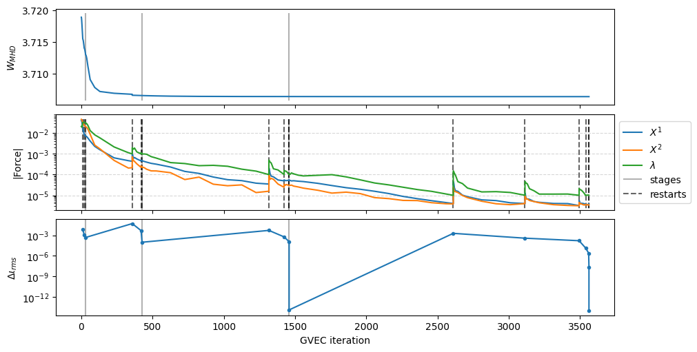
Next we, run GVEC and visualize again the minimization diagnostics:
runpath = "run_current_profile"

run = gvec.run(params, runpath=runpath, keep_intermediates="stages")

fig = run.plot_diagnostics_minimization()
GVEC - completed 0/5 stages, restarts in current stage - 0: |>|.|.|.|.|
GVEC - completed 1/5 stages, restarts in current stage - 0: |=|>|.|.|.|
GVEC - completed 1/5 stages, restarts in current stage - 1: |=|=>|.|.|.|
GVEC - completed 1/5 stages, restarts in current stage - 2: |=|==>|.|.|.|
GVEC - completed 2/5 stages, restarts in current stage - 0: |=|===|>|.|.|
GVEC - completed 2/5 stages, restarts in current stage - 1: |=|===|=>|.|.|
GVEC - completed 2/5 stages, restarts in current stage - 2: |=|===|==>|.|.|
GVEC - completed 3/5 stages, restarts in current stage - 0: |=|===|===|>|.|
GVEC - completed 3/5 stages, restarts in current stage - 1: |=|===|===|=>|.|
GVEC - completed 3/5 stages, restarts in current stage - 2: |=|===|===|==>|.|
GVEC - completed 3/5 stages, restarts in current stage - 3: |=|===|===|===>|.|
GVEC - completed 4/5 stages, restarts in current stage - 0: |=|===|===|====|>|
GVEC - completed 4/5 stages, restarts in current stage - 1: |=|===|===|====|=>|
GVEC - completed 4/5 stages, restarts in current stage - 2: |=|===|===|====|==>|
GVEC - completed 4/5 stages, restarts in current stage - 3: |=|===|===|====|===>|
GVEC - completed 4/5 stages, restarts in current stage - 4: |=|===|===|====|====>|
GVEC - completed 4/5 stages, restarts in current stage - 5: |=|===|===|====|=====>|
GVEC - completed 4/5 stages, restarts in current stage - 6: |=|===|===|====|======>|
GVEC finished after  10.4 seconds  using 3562 iterations (totalIter = 100000)  with |force| = 9.97e-06 (minimize_tol = 1.00e-05)
 and rms Δiota = 9.08e-15(iota_tol=1.00e-10)
Understanding the diagnostics#
As we can see the screen output as well as the visualization has undergone some changes in comparison to the fixed \(\iota\) run. We mentioned above that the underlying algorithm is slightly different. So, what happened here?
GVEC optimizes for \(I_{\text{tor}}\) by adapting \(\iota\) using Picard iterations
\(\iota\) can be split into two major contributions:
one that solely originates from the geometry: \(\iota_0\)
one that also includes contributions from \(I_{\text{tor}}\): \(\iota_{\text{curr}}\)
\(\iota_T = \iota_{\text{curr}} + \iota_0\)
GVEC always runs with fixed \(\iota\) for several iterations before updating \(\iota\) again due to the \(\iota_{\text{curr}}\) contribution
changing the geometry will lead to a discrepancy between \(\iota_T\) and the currently specified \(\iota\):
we track the discrepancy via \(\Delta\iota_{\text{rms}}\)
after a \(\iota\) update GVEC restarts from its previous state with the new profile
picard_currentis used to control the Picard iterations / strategy:the
"auto"mode (recommended) automatically designsstagesdepending on the chosenminimize_tol.
For more theory behind this approach and more advanced control options see the stages section(🌐).
Visualize the result#
Since we optimize for \(I_{\text{tor}}\), small deviations from the prescribed profile are possible. Therefore, let us visualize some of the quantities of interest here:
the toroidal current contribution to the rotational transform \(\iota_{\text{curr}}\) /
iota_currthe final \(\iota\) profile /
iotathe poloidal current
I_polthe toroidal current
I_torcalculated usingiotaand the geometry
For more visualization later on we also calculate p, mod_B, X1 and X2.
First, we have a look at the rotational transform and current profiles, using the plotting function plot_radial_profile(🌐)
fig, axs = run.state.plot_radial_profile(
    ["iota_curr", "iota", "I_tor", "I_pol"]
)
WARNING Computation of `I_pol` uses `rho=1.000000e-04` instead of the magnetic axis.
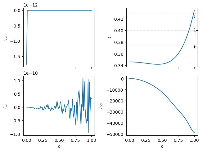
As we can see, the toroidal current calculated from the equilibrium solution, as well as current contribution to the rotational transform, \(\iota_{\text{curr}}\), are almost zero as they should be.
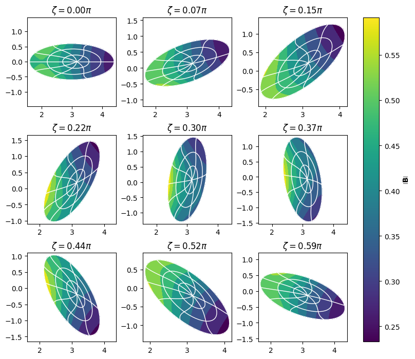
Finally, we can also visualize some of the poloidal cross-sections as before, using plot_poloidal_plane(🌐)
fig, axs = run.state.plot_poloidal_plane(
    plot_kwargs={"figsize": (8, 8)}
)
Summary#
To summarize, for running GVEC with a prescribed current profile one has to set the parameters I_tor and picard_current. Since in this case GVEC updates the rotational transform profile using Picard iterations, small deviations from the prescribed current profile can occur. The parameter picard_current is utilized to control these Picard iterations. Using picard_current="auto" is the recommended approach. Detailed control options can be found in the stages section in the GVEC user guide(🌐).