Boozer transform#
Lets apply the Boozer transform to the equilibrium computed in the tutorial Elliptic Stellarator(🌐).
In GVEC, we use a poloidal angle \(\vartheta\) and toroidal angle \(\zeta\), from which we can easily sample quantities on a regular grid. The transform to Boozer angles is
The Boozer transform is described in the theory section(🌐). In short:
\(\lambda\) is recomputed on a higher Fourier resolution (by default
MNfactor=5is used).\(\nu\) can be deduced from \(\lambda\), and is computed with the same resolution as \(\lambda\).
Evaluations on a regular grid in Boozer angles \((\vartheta_B)_i,(\zeta_B)_j\) means that we have to first find the corresponding \((\vartheta)_{ij},(\zeta)_{ij}\) positions, using a 2D Newton search, and then evaluate on these positions.
import matplotlib.pyplot as plt
import numpy as np

import gvec
Load previously computed state#
We load the state from the previously computed equilibrium by specifying a runpath which we provide to gvec.find_state(🌐).
# path to the previous run
runpath = "run_ellipstell"
state = gvec.find_state(runpath)
Boozer transform#
Now we can construct the grid we want to evaluate on, and call gvec.evaluate_sfl(🌐), which computes the Boozer transform and evaluates on a regular grid in Boozer angles.
nfp = state.nfp
# select 4 radial positions
rho = [0.2, 0.5, 0.8, 1.0]
theta_B = np.linspace(0, 2 * np.pi, 51)
zeta_B = np.linspace(0, 2 * np.pi / nfp, 51)
varlist = [
    "mod_B",
    "B_contra_t",
    "B_contra_z",
    "B_contra_t_B",
    "B_contra_z_B",
]

evb = state.evaluate_sfl(
    *varlist,
    rho=rho,
    theta=theta_B,
    zeta=zeta_B,
    sfl="boozer",
)
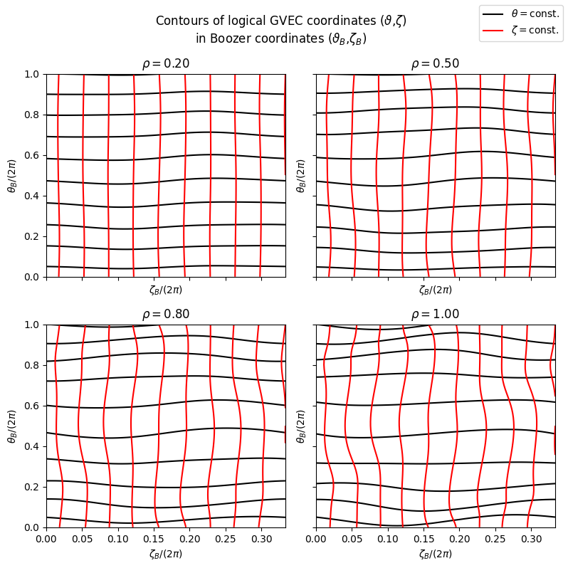
Visualization in Boozer angles#
Lets visualize first the transform as a grid in Boozer angles \(\vartheta_B\) and \(\zeta_B\).
fig, axs = plt.subplots(
    2, 2, figsize=(8, 8), sharey=True, sharex=True, tight_layout=True
)

for i, ax in enumerate(axs.flatten()):
    evi = evb.isel(rad=i)
    ax.contour(
        evi.zeta_B / (2 * np.pi),
        evi.theta_B / (2 * np.pi),
        evi.theta,
        np.linspace(-2 * np.pi, 2 * np.pi, 20),
        colors="black",
    )
    ax.contour(
        evi.zeta_B / (2 * np.pi),
        evi.theta_B / (2 * np.pi),
        evi.zeta,
        np.linspace(-2 * np.pi / 3, 2 * np.pi / 3, 20),
        colors="red",
    )
    ax.set(
        xlabel=r"$\zeta_B/(2\pi)$",
        ylabel=r"$\theta_B/(2\pi)$",
        title=f"$\\rho = {evi.rho.data:.2f}$",
    )
fig.legend(
    handles=[
        plt.Line2D([0], [0], color="black", label=r"$\theta=$const."),
        plt.Line2D([0], [0], color="red", label=r"$\zeta=$const."),
    ]
)
fig.suptitle(
    (
        r"Contours of logical GVEC coordinates ($\vartheta$,$\zeta$)"
        + "\n"
        + r"in Boozer coordinates ($\vartheta_B$,$\zeta_B$)"
    )
)
Text(0.5, 0.98, 'Contours of logical GVEC coordinates ($\\vartheta$,$\\zeta$)\nin Boozer coordinates ($\\vartheta_B$,$\\zeta_B$)')
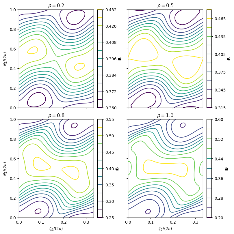
Finally, we can visualise the \(|B|\) contours in Boozer coordinates with the plot_on_flux_surface(🌐) function, on one field period and for multiple flux surfaces.
fig, axs = state.plot_on_flux_surface(
    rho=[0.2, 0.5, 0.8, 1.0], plot_kwargs={"figsize": (8, 8)}
)