Postprocessing#
In this notebook we take a deeper look at postprocessing, using the python interface of GVEC.
GVEC is parallelised with OpenMP and we can set the number of OpenMP threads before importing the gvec package.
import os

os.environ["OMP_NUM_THREADS"] = "2"
This tutorial requires matplotlib to be installed in addition to gvec. numpy and xarray are dependencies of gvec and should therefore be already installed.
import matplotlib.pyplot as plt
import numpy as np
import xarray as xr

import gvec
In this tutorial we will use the equilibrium of the elliptic stellarator, computed in the tutorial Elliptic Stellarator(🌐).
To obtain a gvec.State(🌐) object for this equilibrium, gvec.load_state(🌐) can be used with specific paths for the parameter and statefile.
Alternatively, when each equilibrium is saved in a separate directory, gvec.find_state(🌐) can load the state with only the directory provided.
state = gvec.find_state("./run_ellipstell/")
Derived Quantities#
One of the central features of the GVEC python bindings is the ability to compute a variety of derived quantities.
A list of computable quantities is returned by gvec.table_of_quantities(markdown=True) and also shown at the end of this notebook.
The requested quantities will be stored in an xarray.Dataset, which groups several varaibles, their coordinates and metadata, similar to a pandas Dataframe.
Such a Dataset can also be stored directly as netCDF.
GVEC will also automatically determine which quantities are necessary to compute the desired quantities and add them to the Dataset, thereby also caching them for future computations.
The grid on which the quantities are to be evaluated, can be specified explicitly (with an array or float) or automatically with either an integer for linear spacing (within one field period) or "int" for the integration points required by GVEC.
The state.evaluate(🌐) method can be used to create a new Dataset and compute desired quantities in a single step:
ev = state.evaluate(
    "pos", "B", rho=[0.1, 0.5, 0.9], theta=20, zeta=0.0
)
ev
<xarray.Dataset> Size: 27kB
Dimensions:     (rad: 3, pol: 20, tor: 1, xyz: 3)
Coordinates:
  * rho         (rad) float64 24B 0.1 0.5 0.9
  * theta       (pol) float64 160B 0.0 0.3142 0.6283 ... 5.341 5.655 5.969
  * zeta        (tor) float64 8B 0.0
  * xyz         (xyz) <U1 12B 'x' 'y' 'z'
Dimensions without coordinates: rad, pol, tor
Data variables: (12/44)
    X1          (rad, pol, tor) float64 480B 3.092 3.086 3.068 ... 3.946 4.128
    dX1_dr      (rad, pol, tor) float64 480B 1.217 1.153 0.9674 ... 1.652 1.838
    dX1_dt      (rad, pol, tor) float64 480B 0.0 -0.03914 ... 0.754 0.3979
    dX1_dz      (rad, pol, tor) float64 480B 0.0 0.02456 ... -0.5363 -0.2756
    dX1_drr     (rad, pol, tor) float64 480B -0.02021 -0.06073 ... 3.7 3.349
    dX1_drt     (rad, pol, tor) float64 480B 0.0 -0.4048 ... 0.777 0.4011
    ...          ...
    Jac         (rad, pol, tor) float64 480B 0.2556 0.2549 0.2527 ... 3.559 4.34
    e_theta     (xyz, rad, pol, tor) float64 1kB 0.0 -0.03914 ... 0.4543 0.5512
    e_zeta      (xyz, rad, pol, tor) float64 1kB 0.0 0.02456 ... 1.495 1.643
    B_contra_t  (rad, pol, tor) float64 480B 0.08812 0.08847 ... 0.09179 0.08512
    B_contra_z  (rad, pol, tor) float64 480B 0.1215 0.122 ... 0.06608 0.05889
B (rad, pol, tor, xyz) float64 1kB 0.0 -0.3757 ... -0.2431 0.1437An existing dataset can be extended using state.compute(🌐):
state.compute(ev, "J", "V")
The individual quantities, within an xarray.Dataset can be accessed using ev.B or ev["B"] and are enriched with coordinate information which can be used to a variety of operations, e.g.:
mean_B = ev.B.mean(dim=("rad", "pol", "tor"))
B2 = xr.dot(ev.B, ev.B, dim="xyz")
JxB = xr.cross(ev.J, ev.B, dim="xyz")
Indexing is best done using ev.B.sel(rho=0.5) (by value) or ev.B.isel(rad=0) (by position)
and the raw numpy array can be extracted with ev.B.values.
To ensure a particular order, use ev.B.transpose("rad", "pol", "tor", "xyz").values.
To convert a scalar (e.g. the volume V) into a python scalar use the ev.V.item() method.
The .squeeze() method can be used to remove any dimensions of length 1.
For more information, see the xarray documentation.
Computing integrals#
Specifying "int" for rho, theta and zeta in the Evaluations function, chooses the grid to be the integration points used by GVEC internally.
The functions radial_integral, fluxsurface_integral and volume_integral can then be used to perform integration with the apropriate weights.
E.g. to compute the volume averaged plasma beta, one could use:
ev = state.evaluate(
    "mod_B",
    "mu0",
    "p",
    "Jac",
    "V",
    rho="int",
    theta="int",
    zeta="int",
)
beta = ev.p / (ev.mod_B**2 / (2 * ev.mu0))
beta_avg = gvec.volume_integral(beta * ev.Jac) / ev.V
beta_avg.item()
0.008802419491949296
For supported quantities which require integration (e.g. the volume V computed above), an auxiliary dataset is created to compute them if the grid does not conform to the integration points.
Straight-fieldline coordinates#
GVEC uses flux aligned coordinates (internally also called logical coordinates) \(\rho,\vartheta,\zeta\) to describe the equilibrium.
Available straight fieldline coordinates are PEST- \((\rho,\vartheta_P,\zeta)\) and Boozer coordinates \((\rho,\vartheta_B,\zeta_B)\) for which their associated quantities are denoted with a suffix or subscript P and B respectively.
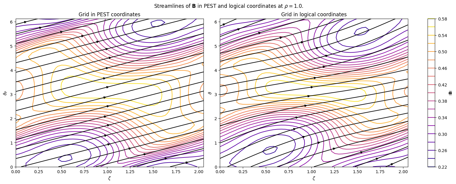
PEST transform#
The PEST coordinates can be computed directly from the GVEC solution with \(\vartheta_P = \vartheta + \lambda(\rho,\vartheta,\zeta)\).
To obtain a grid in PEST coordinates, you can use state.evaluate_sfl(..., sfl="pest")(🌐), which performs a Newton-Raphson search for the respective logical coordinates and then evaluates the requested quantities.
ev = state.evaluate_sfl(
    "mod_B",
    "B_contra_t_P",
    "B_contra_z",  # B_contra_z_P = B_contra_z
    rho=1.0,
    theta=40,
    zeta=50,
    sfl="pest",
).squeeze()

fig, axs = plt.subplots(1, 2, figsize=(15, 6), layout="constrained")
fig.suptitle(
    (
        r"Streamlines of $\mathbf{B}$ in PEST"
        + r" and logical coordinates at $\rho=1.0$."
    )
)

streamplot_kwargs = dict(
    color="black",
    broken_streamlines=False,
    density=1,
    integration_direction="both",
    start_points=np.vstack(
        [
            np.linspace(0, 2 * np.pi / state.nfp, 22)[1:-1],
            np.linspace(2 * np.pi, 0, 22)[1:-1],
        ]
    ).T,
)

ax = axs[0]
c = ax.contour(
    ev.zeta, ev.theta_P, ev.mod_B, levels=21, cmap="plasma"
)
fig.colorbar(
    c, ax=[axs[0], axs[1]], label=f"${ev.mod_B.attrs['symbol']}$"
)
ax.streamplot(
    ev.zeta.values,
    ev.theta_P.values,
    ev.B_contra_z,
    ev.B_contra_t_P,
    **streamplot_kwargs,
)
ax.set_xlabel(r"$\zeta$")
ax.set_ylabel(r"$\vartheta_P$")
ax.set_title("Grid in PEST coordinates")

ev = state.evaluate(
    "mod_B", "B_contra_t", "B_contra_z", rho=1.0, theta=40, zeta=50
).squeeze()

ax = axs[1]
ax.contour(
    ev.zeta, ev.theta, ev.mod_B, levels=21, cmap=c.cmap, norm=c.norm
)
ax.streamplot(
    ev.zeta.values,
    ev.theta.values,
    ev.B_contra_z.values,
    ev.B_contra_t.values,
    **streamplot_kwargs,
)
ax.set_xlabel(r"$\zeta$")
ax.set_ylabel(r"$\vartheta$")
ax.set_title("Grid in logical coordinates")
Text(0.5, 1.0, 'Grid in logical coordinates')
Note
In GVEC the PEST coordinates are generalized also to non-cylindrical coordinates. If a configuration uses a G-Frame or other non-RZφ \(h\)-map, the PEST coordinates retain the toroidal angle \(\zeta\) as defined in the \(h\)-map, which doesn’t necessarily coincide with the cylindrical angle \(\varphi\).
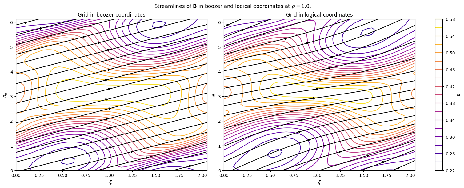
Boozer transform#
To evaluate the equilibrium in Boozer angles, you can use state.evaluate_sfl(..., sfl="boozer")(🌐), which performs a Boozer transform to obtain a set of \(\vartheta,\zeta\) points which correspond to your desired grid in \(\vartheta_B,\zeta_B\).
The evaluations with this new dataset work the same as above, note however that the suffixes t and z still refer to components/derivatives with respect to \(\vartheta,\zeta\).
Some additional quantities, like B_contra_t_B or e_zeta_B are now also available.
The argument MNfactor specifies how many fourier modes should be used for the Boozer potential \(\nu_B\) (and recomputed straight fieldline potential \(\lambda\)) relative to maximum fourier modes used for computing the equilibrium solution.
This parameter has a strong influence on the accuracy and required computational effort!
ev = state.evaluate_sfl(
    "mod_B",
    "B_contra_t_B",
    "B_contra_z_B",
    rho=1.0,
    theta=40,
    zeta=50,
    sfl="boozer",
).squeeze()

fig, axs = plt.subplots(1, 2, figsize=(15, 6), layout="constrained")
fig.suptitle(
    (
        r"Streamlines of $\mathbf{B}$ in boozer"
        + r" and logical coordinates at $\rho=1.0$."
    )
)

streamplot_kwargs = dict(
    color="black",
    broken_streamlines=False,
    density=1,
    integration_direction="both",
    start_points=np.vstack(
        [
            np.linspace(0, 2 * np.pi / state.nfp, 22)[1:-1],
            np.linspace(2 * np.pi, 0, 22)[1:-1],
        ]
    ).T,
)

ax = axs[0]
c = ax.contour(
    ev.zeta_B, ev.theta_B, ev.mod_B, levels=21, cmap="plasma"
)
fig.colorbar(
    c, ax=[axs[0], axs[1]], label=f"${ev.mod_B.attrs['symbol']}$"
)
ax.streamplot(
    ev.zeta_B.values,
    ev.theta_B.values,
    ev.B_contra_z_B,
    ev.B_contra_t_B,
    **streamplot_kwargs,
)
ax.set_xlabel(r"$\zeta_B$")
ax.set_ylabel(r"$\theta_B$")
ax.set_title("Grid in boozer coordinates")

ev = state.evaluate(
    "mod_B", "B_contra_t", "B_contra_z", rho=1.0, theta=40, zeta=50
).squeeze()

ax = axs[1]
ax.contour(
    ev.zeta, ev.theta, ev.mod_B, levels=21, cmap=c.cmap, norm=c.norm
)
ax.streamplot(
    ev.zeta.values,
    ev.theta.values,
    ev.B_contra_z.values,
    ev.B_contra_t.values,
    **streamplot_kwargs,
)
ax.set_xlabel(r"$\zeta$")
ax.set_ylabel(r"$\theta$")
ax.set_title("Grid in logical coordinates")
Text(0.5, 1.0, 'Grid in logical coordinates')
Note
The Boozer transform recomputes \(\lambda\) with a higher resolution (to satisfy the integrability condition for \(\nu_B\))! Therefore some quantities will differ between the equilibrium evaluation and Boozer evaluation.
In particular \(\langle B_\vartheta \rangle, \langle B_\zeta \rangle\) will differ from \(B_{\vartheta_B},B_{\zeta_B}\) by an offset.
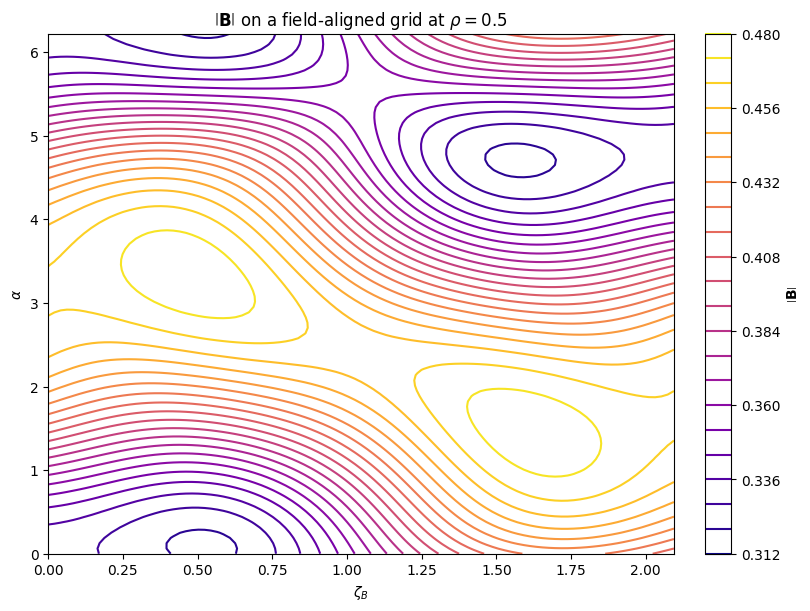
Field-aligned grid#
The state.evaluate_sfl method and EvaluationsBoozer(🌐) ( or EvaluationsPEST(🌐) ) factory function can also be used to generate a non-tensorproduct grid by providing (up to 3D) arrays for the values of \(\theta_B,\zeta_B\).
This can be used for example to create a field-aligned grid:
rho = [0.5, 1.0]  # radial positions
alpha = np.linspace(
    0, 2 * np.pi, 100, endpoint=False
)  # fieldline label
phi = np.linspace(
    0, 2 * np.pi / state.nfp, 101
)  # angle along the fieldline

# evaluate the rotational transform (fieldline angle) on the desired surfaces
iota = state.evaluate("iota", rho=rho, theta=None, zeta=None).iota

# 3D toroidal and poloidal arrays that correspond to fieldline coordinates for each surface
theta_B = (
    alpha[None, :, None]
    + iota.data[:, None, None] * phi[None, None, :]
)

# create the grid
ev = gvec.EvaluationsBoozer(
    rho=rho, theta_B=theta_B, zeta_B=phi, state=state, MNfactor=5
)

# set the fiedline label as poloidal coordinate & index (not necessary, but good practice)
ev["alpha"] = ("pol", alpha)
ev["alpha"].attrs = dict(
    symbol=r"\alpha", long_name="fieldline label"
)
ev = ev.set_coords("alpha").set_xindex("alpha")

state.compute(ev, "B", "B_contra_t_B", "B_contra_z_B", "mod_B")
ev = ev.sel(rho=0.5)

fig, ax = plt.subplots(figsize=(8, 6), layout="constrained")

c = ax.contour(
    ev.zeta_B, ev.alpha, ev.mod_B, levels=21, cmap="plasma"
)
fig.colorbar(c, ax=ax, label=f"${ev.mod_B.attrs['symbol']}$")
ax.set_xlabel(f"${ev.zeta_B.attrs['symbol']}$")
ax.set_ylabel(f"${ev.alpha.attrs['symbol']}$")
ax.set_title(
    (
        f"${ev.mod_B.attrs['symbol']}$"
        + r" on a field-aligned grid at $\rho=0.5$"
    )
)
Text(0.5, 1.0, '$\\left|\\mathbf{B}\\right|$ on a field-aligned grid at $\\rho=0.5$')
Available quantities for evaluation#
The following table contains the quantities that can be evaluated with the python bindings, it can be generated with
gvec.table_of_quantities(markdown=True)
label |
long name |
symbol |
|---|---|---|
|
surface area |
\(A_\text{surface}\) |
|
magnetic field |
\(\mathbf{B}\) |
|
poloidal component of the magnetic field |
\(B^\theta\) |
|
contravariant \(\theta\) component of the magnetic field in Boozer coordinates |
\(B^{\theta_B}\) |
|
contravariant \(\theta\) component of the magnetic field in PEST coordinates |
\(B^{\theta_P}\) |
|
toroidal component of the magnetic field |
\(B^\zeta\) |
|
contravariant \(\zeta\) component of the magnetic field in Boozer coordinates |
\(B^{\zeta_B}\) |
|
\(\rho\) component of the magnetic field in Boozer coordinates |
\(B_{\rho_B}\) |
|
\(\rho\) component of the magnetic field in PEST coordinates |
\(B_{\rho_P}\) |
|
\(\theta\) component of the magnetic field in Boozer coordinates |
\(B_{\theta_B}\) |
|
\(\theta\) component of the magnetic field in PEST coordinates |
\(B_{\theta_P}\) |
|
flux-surface averaged poloidal magnetic field |
\(\overline{B_\theta}\) |
|
\(\zeta\) component of the magnetic field in Boozer coordinates |
\(B_{\zeta_B}\) |
|
\(\zeta\) component of the magnetic field in PEST coordinates |
\(B_{\zeta_P}\) |
|
flux-surface averaged toroidal magnetic field |
\(\overline{B_\zeta}\) |
|
Mercier criterion |
\(D_\text{Merc}\) |
|
Current contribution to the Mercier criterion |
\(D_\text{M,Curr}\) |
|
Geodesic contribution to the Mercier criterion |
\(D_\text{M,Geod}\) |
|
Shear contribution to the Mercier criterion |
\(D_\text{M,Shear}\) |
|
Magnetic well contribution to the Mercier criterion |
\(D_\text{M,Well}\) |
|
MHD force balance |
\(\mathbf{J}\times \mathbf{B}-\nabla p\) |
|
radial force balance |
\(\overline{F_\rho}\) |
|
poloidal component of the second fundamental form |
\(\mathrm{II}_{\theta\theta}\) |
|
t,t component of the second fundamental form in Boozer coordinates |
\(\mathrm{II}_{\theta_B \theta_B}\) |
|
t,t component of the second fundamental form in PEST coordinates |
\(\mathrm{II}_{\theta_P \theta_P}\) |
|
poloidal-toroidal component of the second fundamental form |
\(\mathrm{II}_{\theta\zeta}\) |
|
t,z component of the second fundamental form in Boozer coordinates |
\(\mathrm{II}_{\theta_B \zeta_B}\) |
|
t,z component of the second fundamental form in PEST coordinates |
\(\mathrm{II}_{\theta_P \zeta_P}\) |
|
toroidal component of the second fundamental form |
\(\mathrm{II}_{\zeta\zeta}\) |
|
z,z component of the second fundamental form in Boozer coordinates |
\(\mathrm{II}_{\zeta_B \zeta_B}\) |
|
z,z component of the second fundamental form in PEST coordinates |
\(\mathrm{II}_{\zeta_P \zeta_P}\) |
|
poloidal current, relative to the magnetic axis |
\(I_\text{pol}\) |
|
toroidal current enclosed by flux surface |
\(I_\text{tor}\) |
|
current density |
\(\mathbf{J}\) |
|
contravariant radial current density |
\(J^{\rho}\) |
|
contravariant poloidal current density |
\(J^{\theta}\) |
|
contravariant \(\theta\) component of the current density in Boozer coordinates |
\(J^{\theta_B}\) |
|
contravariant \(\theta\) component of the current density in PEST coordinates |
\(J^{\theta_P}\) |
|
contravariant toroidal current density |
\(J^{\zeta}\) |
|
contravariant \(\zeta\) component of the current density in Boozer coordinates |
\(J^{\zeta_B}\) |
|
\(\rho\) component of the current density in Boozer coordinates |
\(J_{\rho_B}\) |
|
\(\rho\) component of the current density in PEST coordinates |
\(J_{\rho_P}\) |
|
\(\theta\) component of the current density in Boozer coordinates |
\(J_{\theta_B}\) |
|
\(\theta\) component of the current density in PEST coordinates |
\(J_{\theta_P}\) |
|
\(\zeta\) component of the current density in Boozer coordinates |
\(J_{\zeta_B}\) |
|
\(\zeta\) component of the current density in PEST coordinates |
\(J_{\zeta_P}\) |
|
Jacobian determinant |
\(\mathcal{J}\) |
|
Jacobian determinant in Boozer coordinates |
\(\mathcal{J}_B\) |
|
Jacobian determinant in PEST coordinates |
\(\mathcal{J}_P\) |
|
reference Jacobian determinant |
\(\mathcal{J}_h\) |
|
logical Jacobian determinant |
\(\mathcal{J}_l\) |
|
straight field line potential |
\(\lambda\) |
|
length of the magnetic axis |
\(L_\text{axis}\) |
|
magnetic gradient scale length |
\(L_{\nabla\mathbf{B}}\) |
|
number of field periods |
\(N_\text{FP}\) |
|
toroidal magnetic flux |
\(\Phi\) |
|
toroidal magnetic flux at the edge |
\(\Phi_0\) |
|
volume |
\(V\) |
|
total MHD energy |
\(W_\text{MHD}\) |
|
first reference coordinate |
\(X^1\) |
|
second reference coordinate |
\(X^2\) |
|
effective aspect ratio |
\(a_\text{eff}\) |
|
volume-averaged plasma beta |
\(\overline{\beta}\) |
|
poloidal magnetic flux |
\(\chi\) |
|
differential area element |
\(dA\) |
|
radial derivative of the poloidal magnetic field |
\(\frac{\partial B^\theta}{\partial \rho}\) |
|
poloidal derivative of the poloidal magnetic field |
\(\frac{\partial B^\theta}{\partial \theta}\) |
|
toroidal derivative of the poloidal magnetic field |
\(\frac{\partial B^\theta}{\partial \zeta}\) |
|
radial derivative of the toroidal magnetic field |
\(\frac{\partial B^\zeta}{\partial \rho}\) |
|
poloidal derivative of the toroidal magnetic field |
\(\frac{\partial B^\zeta}{\partial \theta}\) |
|
toroidal derivative of the toroidal magnetic field |
\(\frac{\partial B^\zeta}{\partial \zeta}\) |
|
radial derivative of the magnetic field |
\(\frac{\partial \mathbf{B}}{\partial \rho}\) |
|
poloidal derivative of the magnetic field |
\(\frac{\partial \mathbf{B}}{\partial \theta}\) |
|
toroidal derivative of the magnetic field |
\(\frac{\partial \mathbf{B}}{\partial \zeta}\) |
|
derivative of the flux-surface averaged poloidal magnetic field |
\(\frac{d\overline{B_\theta}}{d\rho}\) |
|
derivative of the toroidal current enclosed by the flux surface |
\(\frac{dI_\text{tor}}{d\rho}\) |
|
radial derivative of the Jacobian determinant |
\(\frac{\partial \mathcal{J}}{\partial \rho}\) |
|
poloidal derivative of the Jacobian determinant |
\(\frac{\partial \mathcal{J}}{\partial \theta}\) |
|
toroidal derivative of the Jacobian determinant |
\(\frac{\partial \mathcal{J}}{\partial \zeta}\) |
|
radial derivative of the reference Jacobian determinant |
\(\frac{\partial \mathcal{J}_h}{\partial \rho}\) |
|
poloidal derivative of the reference Jacobian determinant |
\(\frac{\partial \mathcal{J}_h}{\partial \theta}\) |
|
toroidal derivative of the reference Jacobian determinant |
\(\frac{\partial \mathcal{J}_h}{\partial \zeta}\) |
|
radial derivative of the logical Jacobian determinant |
\(\frac{\partial \mathcal{J}_l}{\partial \rho}\) |
|
poloidal derivative of the logical Jacobian determinant |
\(\frac{\partial \mathcal{J}_l}{\partial \theta}\) |
|
toroidal derivative of the logical Jacobian determinant |
\(\frac{\partial \mathcal{J}_l}{\partial \zeta}\) |
|
radial derivative of the straight field line potential |
\(\frac{\partial \lambda}{\partial \rho}\) |
|
second radial derivative of the straight field line potential |
\(\frac{\partial^2 \lambda}{\partial \rho^2}\) |
|
radial-poloidal derivative of the straight field line potential |
\(\frac{\partial^2 \lambda}{\partial \rho\partial \theta}\) |
|
radial-toroidal derivative of the straight field line potential |
\(\frac{\partial^2 \lambda}{\partial \rho\partial \zeta}\) |
|
poloidal derivative of the straight field line potential |
\(\frac{\partial \lambda}{\partial \theta}\) |
|
second poloidal derivative of the straight field line potential |
\(\frac{\partial^2 \lambda}{\partial \theta^2}\) |
|
poloidal-toroidal derivative of the straight field line potential |
\(\frac{\partial^2 \lambda}{\partial \theta\partial \zeta}\) |
|
toroidal derivative of the straight field line potential |
\(\frac{\partial \lambda}{\partial \zeta}\) |
|
second toroidal derivative of the straight field line potential |
\(\frac{\partial^2 \lambda}{\partial \zeta^2}\) |
|
poloidal derivative of the Boozer potential computed from the magnetic field |
\(\left.\frac{\partial \nu_B}{\partial \theta}\right|_\text{def.}\) |
|
toroidal derivative of the Boozer potential computed from the magnetic field |
\(\left.\frac{\partial \nu_B}{\partial \zeta}\right|_\text{def.}\) |
|
toroidal magnetic flux gradient |
\(\frac{d\Phi}{d\rho}\) |
|
toroidal magnetic flux curvature |
\(\frac{d^2\Phi}{d\rho^2}\) |
|
derivative of the plasma volume w.r.t. normalized toroidal magnetic flux |
\(\frac{dV}{d\Phi_n}\) |
|
second derivative of the plasma volume w.r.t. normalized toroidal magnetic flux |
\(\frac{d^2V}{d\Phi_n^2}\) |
|
radial derivative of the first reference coordinate |
\(\frac{\partial X^1}{\partial \rho}\) |
|
second radial derivative of the first reference coordinate |
\(\frac{\partial^2 X^1}{\partial \rho^2}\) |
|
radial-poloidal derivative of the first reference coordinate |
\(\frac{\partial^2 X^1}{\partial \rho\partial \theta}\) |
|
radial-toroidal derivative of the first reference coordinate |
\(\frac{\partial^2 X^1}{\partial \rho\partial \zeta}\) |
|
poloidal derivative of the first reference coordinate |
\(\frac{\partial X^1}{\partial \theta}\) |
|
second poloidal derivative of the first reference coordinate |
\(\frac{\partial^2 X^1}{\partial \theta^2}\) |
|
poloidal-toroidal derivative of the first reference coordinate |
\(\frac{\partial^2 X^1}{\partial \theta\partial \zeta}\) |
|
toroidal derivative of the first reference coordinate |
\(\frac{\partial X^1}{\partial \zeta}\) |
|
second toroidal derivative of the first reference coordinate |
\(\frac{\partial^2 X^1}{\partial \zeta^2}\) |
|
radial derivative of the second reference coordinate |
\(\frac{\partial X^2}{\partial \rho}\) |
|
second radial derivative of the second reference coordinate |
\(\frac{\partial^2 X^2}{\partial \rho^2}\) |
|
radial-poloidal derivative of the second reference coordinate |
\(\frac{\partial^2 X^2}{\partial \rho\partial \theta}\) |
|
radial-toroidal derivative of the second reference coordinate |
\(\frac{\partial^2 X^2}{\partial \rho\partial \zeta}\) |
|
poloidal derivative of the second reference coordinate |
\(\frac{\partial X^2}{\partial \theta}\) |
|
second poloidal derivative of the second reference coordinate |
\(\frac{\partial^2 X^2}{\partial \theta^2}\) |
|
poloidal-toroidal derivative of the second reference coordinate |
\(\frac{\partial^2 X^2}{\partial \theta\partial \zeta}\) |
|
toroidal derivative of the second reference coordinate |
\(\frac{\partial X^2}{\partial \zeta}\) |
|
second toroidal derivative of the second reference coordinate |
\(\frac{\partial^2 X^2}{\partial \zeta^2}\) |
|
radial derivative of the normalized magnetic field |
\(\frac{\partial \mathbf{b}}{\partial \rho}\) |
|
poloidal derivative of the normalized magnetic field |
\(\frac{\partial \mathbf{b}}{\partial \theta}\) |
|
toroidal derivative of the normalized magnetic field |
\(\frac{\partial \mathbf{b}}{\partial \zeta}\) |
|
poloidal magnetic flux gradient |
\(\frac{d\chi}{d\rho}\) |
|
poloidal magnetic flux curvature |
\(\frac{d^2\chi}{d\rho^2}\) |
|
radial derivative of the rr component of the metric tensor |
\(\frac{\partial g_{\rho\rho}}{\partial \rho}\) |
|
poloidal derivative of the rr component of the metric tensor |
\(\frac{\partial g_{\rho\rho}}{\partial \theta}\) |
|
toroidal derivative of the rr component of the metric tensor |
\(\frac{\partial g_{\rho\rho}}{\partial \zeta}\) |
|
radial derivative of the rt component of the metric tensor |
\(\frac{\partial g_{\rho\theta}}{\partial \rho}\) |
|
poloidal derivative of the rt component of the metric tensor |
\(\frac{\partial g_{\rho\theta}}{\partial \theta}\) |
|
toroidal derivative of the rt component of the metric tensor |
\(\frac{\partial g_{\rho\theta}}{\partial \zeta}\) |
|
radial derivative of the rz component of the metric tensor |
\(\frac{\partial g_{\rho\zeta}}{\partial \rho}\) |
|
poloidal derivative of the rz component of the metric tensor |
\(\frac{\partial g_{\rho\zeta}}{\partial \theta}\) |
|
toroidal derivative of the rz component of the metric tensor |
\(\frac{\partial g_{\rho\zeta}}{\partial \zeta}\) |
|
radial derivative of the tt component of the metric tensor |
\(\frac{\partial g_{\theta\theta}}{\partial \rho}\) |
|
poloidal derivative of the tt component of the metric tensor |
\(\frac{\partial g_{\theta\theta}}{\partial \theta}\) |
|
toroidal derivative of the tt component of the metric tensor |
\(\frac{\partial g_{\theta\theta}}{\partial \zeta}\) |
|
radial derivative of the tz component of the metric tensor |
\(\frac{\partial g_{\theta\zeta}}{\partial \rho}\) |
|
poloidal derivative of the tz component of the metric tensor |
\(\frac{\partial g_{\theta\zeta}}{\partial \theta}\) |
|
toroidal derivative of the tz component of the metric tensor |
\(\frac{\partial g_{\theta\zeta}}{\partial \zeta}\) |
|
radial derivative of the zz component of the metric tensor |
\(\frac{\partial g_{\zeta\zeta}}{\partial \rho}\) |
|
poloidal derivative of the zz component of the metric tensor |
\(\frac{\partial g_{\zeta\zeta}}{\partial \theta}\) |
|
toroidal derivative of the zz component of the metric tensor |
\(\frac{\partial g_{\zeta\zeta}}{\partial \zeta}\) |
|
rotational transform gradient |
\(\frac{d\iota}{d\rho}\) |
|
rotational transform curvature |
\(\frac{d^2\iota}{d\rho^2}\) |
|
radial derivative of the modulus of the magnetic field |
\(\frac{\partial \left|\mathbf{B}\right|}{\partial \rho}\) |
|
radial Boozer derivative of the modulus of the magnetic field |
\(\frac{\partial\left|\mathbf{B}\right|}{\partial \rho_B}\) |
|
radial PEST-like derivative of the modulus of the magnetic field |
\(\frac{\partial\left|\mathbf{B}\right|}{\partial \rho_P}\) |
|
poloidal derivative of the modulus of the magnetic field |
\(\frac{\partial \left|\mathbf{B}\right|}{\partial \theta}\) |
|
poloidal Boozer derivative of the modulus of the magnetic field |
\(\frac{\partial\left|\mathbf{B}\right|}{\partial \theta_B}\) |
|
poloidal PEST-like derivative of the modulus of the magnetic field |
\(\frac{\partial\left|\mathbf{B}\right|}{\partial \vartheta_P}\) |
|
toroidal derivative of the modulus of the magnetic field |
\(\frac{\partial \left|\mathbf{B}\right|}{\partial \zeta}\) |
|
toroidal Boozer derivative of the modulus of the magnetic field |
\(\frac{\partial\left|\mathbf{B}\right|}{\partial \zeta_B}\) |
|
toroidal PEST-like derivative of the modulus of the magnetic field |
\(\frac{\partial\left|\mathbf{B}\right|}{\partial \zeta_P}\) |
|
pressure gradient |
\(\frac{dp}{d\rho}\) |
|
pressure curvature |
\(\frac{d^2p}{d\rho^2}\) |
|
first reference tangent basis vector |
\(\mathbf{e}_{q^1}\) |
|
second reference tangent basis vector |
\(\mathbf{e}_{q^2}\) |
|
toroidal reference tangent basis vector |
\(\mathbf{e}_{q^3}\) |
|
radial tangent basis vector |
\(\mathbf{e}_\rho\) |
|
radial tangent basis vector in Boozer coordinates |
\(\mathbf{e}_{\rho_B}\) |
|
poloidal tangent basis vector in PEST coordinates |
\(\mathbf{e}_{\theta_P}\) |
|
poloidal tangent basis vector |
\(\mathbf{e}_\theta\) |
|
poloidal tangent basis vector in Boozer coordinates |
\(\mathbf{e}_{\theta_B}\) |
|
poloidal tangent basis vector in PEST coordinates |
\(\mathbf{e}_{\theta_P}\) |
|
toroidal tangent basis vector |
\(\mathbf{e}_\zeta\) |
|
toroidal tangent basis vector in Boozer coordinates |
\(\mathbf{e}_{\zeta_B}\) |
|
toroidal tangent basis vector in PEST coordinates |
\(\mathbf{e}_{\zeta_P}\) |
|
effective elongation |
\(E_\text{eff}\) |
|
rr component of the metric tensor |
\(g_{\rho\rho}\) |
|
rr component of the metric tensor in Boozer coordinates |
\(g_{\rho_B \rho_B}\) |
|
rr component of the metric tensor in PEST coordinates |
\(g_{\rho_P \rho_P}\) |
|
rt component of the metric tensor |
\(g_{\rho\theta}\) |
|
rt component of the metric tensor in Boozer coordinates |
\(g_{\rho_B \theta_B}\) |
|
rt component of the metric tensor in PEST coordinates |
\(g_{\rho_P \theta_P}\) |
|
rz component of the metric tensor |
\(g_{\rho\zeta}\) |
|
rz component of the metric tensor in Boozer coordinates |
\(g_{\rho_B \zeta_B}\) |
|
rz component of the metric tensor in PEST coordinates |
\(g_{\rho_P \zeta_P}\) |
|
tt component of the metric tensor |
\(g_{\theta\theta}\) |
|
tt component of the metric tensor in Boozer coordinates |
\(g_{\theta_B \theta_B}\) |
|
tt component of the metric tensor in PEST coordinates |
\(g_{\theta_P \theta_P}\) |
|
tz component of the metric tensor |
\(g_{\theta\zeta}\) |
|
tz component of the metric tensor in Boozer coordinates |
\(g_{\theta_B \zeta_B}\) |
|
tz component of the metric tensor in PEST coordinates |
\(g_{\theta_P \zeta_P}\) |
|
zz component of the metric tensor |
\(g_{\zeta\zeta}\) |
|
zz component of the metric tensor in Boozer coordinates |
\(g_{\zeta_B \zeta_B}\) |
|
zz component of the metric tensor in PEST coordinates |
\(g_{\zeta_P \zeta_P}\) |
|
adiabatic index |
\(\gamma\) |
|
volume-averaged gradient of magnetic pressure |
\(\left\langle\left|\nabla\frac{B^2}{2\mu_0}\right|\right\rangle_\text{vol}\) |
|
gradient of the modulus of the magnetic field |
\(\nabla\left|\mathbf{B}\right|\) |
|
radial reciprocal basis vector |
\(\nabla\rho\) |
|
poloidal reciprocal basis vector |
\(\nabla\theta\) |
|
poloidal reciprocal basis vector in Boozer coordinates |
\(\nabla\theta_B\) |
|
poloidal reciprocal basis vector in PEST coordinates |
\(\nabla \theta_P\) |
|
toroidal reciprocal basis vector |
\(\nabla\zeta\) |
|
toroidal reciprocal basis vector in Boozer coordinates |
\(\nabla\zeta_B\) |
|
rotational transform |
\(\iota\) |
|
geometric contribution to the rotational transform |
\(\iota_0\) |
|
average rotational transform |
\(\overline{\iota}\) |
|
rotational transform averaged over rho^2 |
\(\overline{\iota}_2\) |
|
toroidal current contribution to the rotational transform |
\(\iota_\text{curr}\) |
|
factor to the toroidal current contribution to the rotational transform |
\(\iota_{\text{curr},0}\) |
|
q1-q1 reference curvature vector |
\(k_{q^1q^1}\) |
|
q1-q2 reference curvature vector |
\(k_{q^1q^2}\) |
|
q1-q3 reference curvature vector |
\(k_{q^1q^3}\) |
|
q2-q2 reference curvature vector |
\(k_{q^2q^2}\) |
|
q2-q3 reference curvature vector |
\(k_{q^2q^3}\) |
|
q3-q3 reference curvature vector |
\(k_{q^3q^3}\) |
|
rr logical curvature vector |
\(\mathbf{k}_{\rho\rho}\) |
|
rt logical curvature vector |
\(\mathbf{k}_{\rho\theta}\) |
|
rz logical curvature vector |
\(\mathbf{k}_{\rho\zeta}\) |
|
tt logical curvature vector |
\(\mathbf{k}_{\theta\theta}\) |
|
tt boozer curvature vector |
\(\mathbf{k}_{\theta_B \theta_B}\) |
|
tt PEST curvature vector |
\(\mathbf{k}_{\theta_P \theta_P}\) |
|
tz logical curvature vector |
\(\mathbf{k}_{\theta\zeta}\) |
|
tz boozer curvature vector |
\(\mathbf{k}_{\theta_B \zeta_B}\) |
|
tz PEST curvature vector |
\(\mathbf{k}_{\theta_P \zeta_P}\) |
|
zz logical curvature vector |
\(\mathbf{k}_{\zeta\zeta}\) |
|
zz boozer curvature vector |
\(\mathbf{k}_{\zeta_B \zeta_B}\) |
|
zz PEST curvature vector |
\(\mathbf{k}_{\zeta_P \zeta_P}\) |
|
field line curvature vector |
\(\mathbf{\kappa}_B\) |
|
geodesic curvature |
\(\kappa_G\) |
|
normal curvature |
\(\kappa_N\) |
|
mirror ratio |
\(\Delta_\text{mirror}\) |
|
modulus of the magnetic field |
\(\left|\mathbf{B}\right|\) |
|
modulus of the MHD force balance |
\(\left|\mathbf{J}\times \mathbf{B}-\nabla p\right|\) |
|
relative MHD force balance |
\(\frac{|\mathbf{J}\times\mathbf{B}-\nabla p|}{\left\langle\left|\nabla(B^2/2\mu_0)\right|\right\rangle_\text{vol}}\) |
|
flux surface average of the relative MHD force balance |
\(\frac{\left\langle|\mathbf{J}\times\mathbf{B}-\nabla p|\right\rangle_\text{surf}}{\left\langle\left|\nabla(B^2/2\mu_0)\right|\right\rangle_\text{vol}}\) |
|
volume average of the relative MHD force balance |
\(\frac{\left\langle|\mathbf{J}\times\mathbf{B}-\nabla p|\right\rangle_\text{vol}}{\left\langle\left|\nabla(B^2/2\mu_0)\right|\right\rangle_\text{vol}}\) |
|
modulus of the current density |
\(\left|\mathbf{J}\right|\) |
|
modulus of the radial tangent basis vector |
\(\left|\mathbf{e}_\rho\right|\) |
|
modulus of the poloidal tangent basis vector |
\(\left|\mathbf{e}_\theta\right|\) |
|
modulus of the toroidal tangent basis vector |
\(\left|\mathbf{e}_\zeta\right|\) |
|
modulus of the radial reciprocal basis vector |
\(\left|\nabla\rho\right|\) |
|
modulus of the poloidal reciprocal basis vector |
\(\left|\nabla\theta\right|\) |
|
modulus of the toroidal reciprocal basis vector |
\(\left|\nabla\zeta\right|\) |
|
magnetic constant |
\(\mu_0\) |
|
surface normal |
\(\mathbf{n}\) |
|
pressure |
\(p\) |
|
position vector |
\(\mathbf{x}\) |
|
effective major radius |
\(r_\text{major,eff}\) |
|
effective minor radius |
\(r_\text{minor,eff}\) |
|
global magnetic shear |
\(s_g\) |
|
average global magnetic shear |
\(\overline{s_g}\) |
|
global magnetic shear averaged over rho^2 |
\(\overline{s_g}_2\) |
|
poloidal angle in PEST coordinates |
\(\theta_P\) |
|
vacuum magnetic well depth |
\(d_\text{well}\) |
|
cartesian vector components |
\((x,y,z)\) |