Coordinate conventions

GVEC coordinates

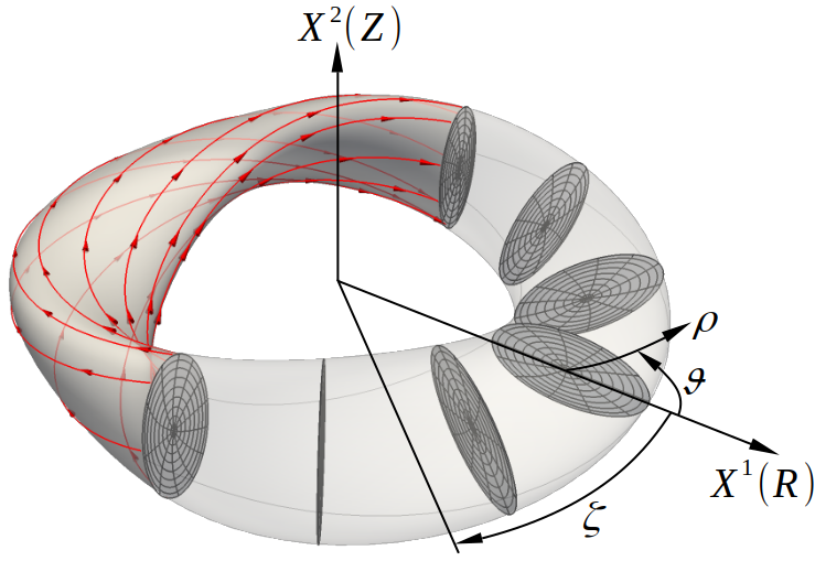
Sketch of the GVEC logical coordinate directions \(\rho,\vartheta,\zeta\) in a stellarator geometry (with magnetic field lines shown in red).

GVEC uses a flux aligned coordinate system with a radial coordinate \(\rho\in[0,1]\), proportional to the square root of the normalized toroidal flux, and two angular coordinates \(\vartheta,\zeta\in[0,2\pi]\). The Boozer-straight-fieldline-angles \(\vartheta_B,\zeta_B\in[0,2\pi]\) are a different set of flux aligned coordinates.

GVEC uses right-handed \((\rho,\vartheta,\zeta)\) and \((\rho,\vartheta_B,\zeta_B)\) systems with the poloidal angles \(\vartheta,\vartheta_B\) increasing clockwise in the poloidal plane (of constant \(\zeta\) or \(\zeta_B\)). GVEC also uses a right-handed \((X^1,X^2,\zeta)\) reference coordinate frame, e.g. a cylindrical coordinate system \((R,Z,\zeta)\). Note that this definition of the cylindrical coordinate system has the toroidal angle \(\zeta\) increasing clockwise when viewing the \(R,Z\)-plane from above.

Different conventions

Assuming another code uses flux aligned coordinates \((s,u,v)\) with different conventions, i.e.

\(\qquad s=s(\rho)\,, \quad u=u(\vartheta)\,, \quad v=v(\zeta)\quad\) or

\(\qquad s=s(\rho)\,, \quad u=u(\vartheta_B)\,, \quad v=v(\zeta_B)\,.\)

In the following we will assume logical flux aligned coordinates \((\rho,\vartheta,\zeta)\), but the same formulas apply if one replaces \(\vartheta,\zeta\) by Boozer straight-fieldline-angles \(\vartheta_B,\zeta_B\).

From the relations \(s(\rho), u(\vartheta)\) and \(v(\zeta)\) we get the derivatives \(\frac{ds}{d\rho},\frac{du}{d\vartheta},\frac{dv}{d\zeta}\).

Geometric Quantities

reciprocal basis vectors

\[\begin{split} \begin{align} \boldsymbol{e}_s &:=\frac{\partial\boldsymbol{x}}{\partial s} & &= \left(\frac{ds}{d\rho}\right)^{-1} \boldsymbol{e}_\rho \\ \boldsymbol{e}_u &:=\frac{\partial\boldsymbol{x}}{\partial u} & &= \left(\frac{du}{d\vartheta}\right)^{-1} \boldsymbol{e}_\vartheta \\ \boldsymbol{e}_v &:=\frac{\partial\boldsymbol{x}}{\partial v} & &= \left(\frac{dv}{d\zeta}\right)^{-1} \boldsymbol{e}_\zeta \end{align} \end{split}\]

contravariant components of a vector \(\boldsymbol{Q}\)

\[\begin{split} \begin{align} Q^{s} &= \frac{ds}{d\rho} Q^{\rho} \\ Q^{u} &= \frac{du}{d\vartheta} Q^{u} \\ Q^{v} &= \frac{dv}{d\zeta} Q^{\zeta} \end{align} \end{split}\]

Jacobian determinant

\[ \mathcal{J} :=\boldsymbol{e}_{s}\cdot\boldsymbol{e}_{u}\times\boldsymbol{e}_{\zeta} = \left(\frac{ds}{d\rho}\frac{du}{d\vartheta}\frac{dv}{d\zeta}\right)^{-1} \mathcal{J}_{\rho\vartheta\zeta} \]

components of the metric tensor

\[\begin{split} \begin{align} g_{ss} &:=\boldsymbol{e}_{s}\cdot\boldsymbol{e}_{s} &&= \left(\frac{ds}{d\rho}\right)^{-2} g_{\rho\rho} \\ g_{su} &&&= \left(\frac{ds}{d\rho}\frac{du}{d\vartheta}\right)^{-1} g_{\rho\vartheta} \\ g_{sv} &&&= \left(\frac{ds}{d\rho}\frac{dv}{d\zeta}\right)^{-1} g_{\rho\zeta} \\ g_{uu} &&&= \left(\frac{du}{d\vartheta}\right)^{-2} g_{\vartheta\vartheta} \\ g_{uv} &&&= \left(\frac{du}{d\vartheta}\frac{dv}{d\zeta}\right)^{-1} g_{\vartheta\zeta} \\ g_{vv} &&&= \left(\frac{dv}{d\zeta}\right)^{-2} g_{\zeta\zeta} \end{align} \end{split}\]

components of the second fundamental form (of the fluxsurfaces)

\[\begin{split} \begin{align} \mathrm{II}_{uu} &:= \boldsymbol{n}\cdot\frac{\partial^{2}\boldsymbol{x}}{\partial u^{2}} &&= \left(\frac{du}{d\vartheta}\right)^{-2} \mathrm{II}_{\vartheta\vartheta} \\ \mathrm{II}_{uv} &&&= \left(\frac{du}{d\vartheta}\frac{dv}{d\zeta}\right)^{-1} \mathrm{II}_{\vartheta\zeta} \\ \mathrm{II}_{vv} &&&= \left(\frac{dv}{d\zeta}\right)^{-2} \mathrm{II}_{\zeta\zeta} \end{align} \end{split}\]