Elliptic Tokamak

In this tutorial GVEC is used to compute and visualize the equilibrium of an elliptic tokamak.

The notebook covers the following steps:

1. Explaining the GVEC input parameters

2. Running GVEC from the notebook

3. Loading the solution for post-processing

4. Evaluating equilibrium quantities and visualize them

5. Running pygvec on the command line

# set the number of OpenMP threads before importing gvec
import os

os.environ["OMP_NUM_THREADS"] = "2"

import numpy as np
import matplotlib.pyplot as plt

import gvec

Setting up a GVEC run

In this example, we first define the parameters in a dictionary.

The full list of parameters is found here.

params = {}
# Project name is used in output files
params["ProjectName"] = "GVEC_elliptok"

Problem setup

For a fixed-boundary MHD equilibrium problem, one needs to specify:

• the physics parameters and

• boundary shape.

In addition, we will also have to provide some numerical parameters for the solver.

Physics parameters

The required physics parameters for a GVEC run are:

• The scale of the magnetic field strength is set by the total enclosed torodial flux \(\Phi_\text{edge}\).

• Rotational transform \(\iota(s)\) and pressure \(p(s)\) profiles. These can be specified in different ways. For example here we define,

  • rotational transform (iota) by providing the coefficients (coefs) of a polynomial in \(s\) and

  • pressure (pres) by specifying the values (vals) at given \(s\) positions (rho2), which are then used to construct a continuous pressure profile using interpolation by a cubic spline.

    • Additionally, the profile can be scaled by a factor scale.

Note that these profiles are always defined in terms of the normalized toroidal flux: \(s=\Phi/\Phi_\text{edge}=\rho^2\)

# total enclosed toroidal flux (scales magnetic field stength)
params["PhiEdge"] = 1.0
# rotational transform profile
params["iota"] = {
    "type": "polynomial",  # c_0 + c_1*s + c_2*s^2 ..., s=rho^2
    "coefs": [0.625, 0.35],  # [c_0,c_1]
}
# pressure profile
params["pres"] = {
    "type": "interpolation",
    "rho2": [0.0, 0.25, 0.5, 0.75, 1.0],  # s=rho^2 positions
    "vals": [1.0, 0.75, 0.5, 0.25, 0.0],  # pressure values at the rho^2 positions
    "scale": 1000.0,  # scaling factor
}

Boundary shape

We first specify the geometry of the equilibrium. For the boundary we need:

• The choice of \(h\)-map.

  For this case we use cylindrical coordinates, so we choose which_hmap=1, so that the mapping to Cartesian coordinates is,

  \[(x,y,z) \mapsto (R\cos(\zeta), -R\sin(\zeta), Z), \qquad \text{with}\qquad R = X^1,\; Z = X^2.\]

• The coefficients corresponding to the \((m,n)\) toroidal and poloidal cosine/sine Fourier modes of \(X^1\) and \(X^2\),

  \[\begin{align*} X^1(\vartheta,\zeta) &= X^1_{0,0} + X^1_{1,0} \cos(\vartheta) + \dots + X^1_{m,n} \cos(m\vartheta - n N_{FP} \zeta), \\ X^2(\vartheta,\zeta) &= \phantom{X^1_{0,0} + {}} X^2_{1,0} \sin(\vartheta) + \dots + X^2_{m,n} \sin(m\vartheta - n N_{FP} \zeta)\,. \end{align*}\]

  • Note that we only specify the \(m\le1\), \(n=0\) modes in this case.

  • The number of toroidal field periods \(N_{FP}\), which in this case is nfp=1.

# set hmap to cylinder coordindates: X1=R,X2=Z,zeta=-phi
params["which_hmap"] = 1
# number of field periods
params["nfp"] = 1
# boundary modes
params["X1_b_cos"] = {
    (0, 0): 5.0,
    (1, 0): 0.9,
}
params["X2_b_sin"] = {(1, 0): 1.1}

Numerical setup

Finally, we must specify some parameters for the numerics.

• The initial guess for the magnetic axis given as the \((m,n)\) Fourier modes for \(X^1\) and \(X^2\) at \(\rho=0\).

• The Fourier resolution in the toroidal \(m\) and poloidal \(n\) directions for the solution parameters \(X^1\), \(X^2\) and \(\lambda\) (X1_mn_max,X2_mn_max,LA_mn_max).

  • Note that this can be larger or smaller than maximum mode number of the boundary. If it is smaller it will cut off the boundary modes at the specified resolution.

• Discretization parameters for the radial B-splines which are

  • the number of radial elements sgrid_nElems for all solution quantities. NOTE using \(\ge2\) elements is recommended;

  • the degree of the B-splines, separately for \(X^1,X^2\) (X1X2_deg) and \(\lambda\) (LA_deg).

  The number of degrees of freedom for a B-spline is nElems + deg. Note that one can change the grid spacing, but here we leave it as the default, which is a uniform spacing in \(\rho\).

• Minimization parameters

  • Maximum number of iterations (totalIter).

  • The tolerance for the minimizer, used as a stopping criterion. The minimization is stopped if \(\max(\|F_{X^1}\|_2,\|F_{X^2}\|_2,\|F_{\lambda}\|_2)\leq \) minimize_tol, where the \(F\) are the forces in the respective solution variable.

# initial guess for magnetic axis
params["X1_a_cos"] = {(0, 0): 5.0}

# maximum Fourier mode numbers for X1,X2,LA [m:poloidal,n:toroidal]
params["X1_mn_max"] = [3, 0]
params["X2_mn_max"] = [3, 0]
params["LA_mn_max"] = [3, 0]

# radial resolution parameters
# number of radial B-spline elements
params["sgrid_nElems"] = 2
# degree of B-splines for X1 and X2
params["X1X2_deg"] = 5
# degree of B-splines for LA
params["LA_deg"] = 5

# minimizer parameters
# maximum number of iterations
params["totalIter"] = 10000
# stopping tolerance in the energy minimization
params["minimize_tol"] = 1e-6

---

Running GVEC

We now have all the parameters in a dictionary params, which we can pass to gvec.run to compute the MHD equilibrium.

The output is stored in the run object.

run = gvec.run(params, runpath="run_tokamak")

GVEC: |>|
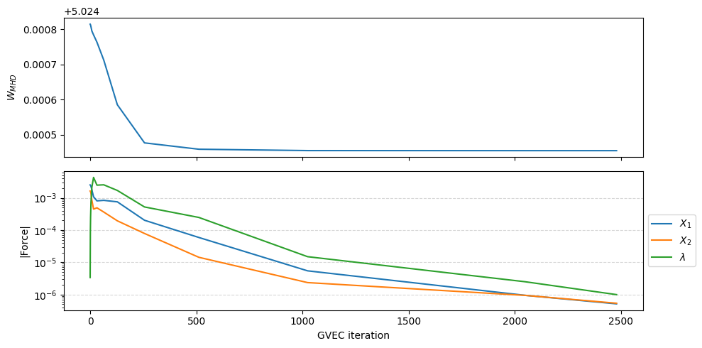
GVEC finished after   0.5 seconds  using 2479 iterations (totalIter = 10000)  with |force| = 9.97e-07 (minimize_tol = 1.00e-06)

We can extract and plot the history of the GVEC run. We see the change in total MHD energy and the norm of the forces, which are computed as \(\|F\|_2\) for each unknown \(X^1,X^2,\lambda\).

fig = run.plot_diagnostics_minimization()

---

Post-processing

The central object for evaluating a GVEC equilibrium is the gvec.State class.

One can load the final state file from the object run that was the output of gvec.run.

Alternatively, if the run was done outside this notebook, we can find the state from a runpath using gvec.find_state(runpath).

state = run.state

Evaluate the equilibrium state

Choose a discrete set of 1D points in radial direction rho (proportional to the square-root of the magnetic flux) and poloidal direction theta and toroidal direction zeta.

• Either by specifying an array, or just the number of points.

• As this example is a tokamak, only one point in zeta is used.

The data is stored in ev, which is an xarray.Dataset.

rho = np.linspace(0, 1, 20)  # radial visualization points
theta = np.linspace(0, 2 * np.pi, 50)  # poloidal visualization points

ev = state.evaluate("X1", "X2", "LA", "iota", "p", rho=rho, theta=theta, zeta=[0.0])

Visualize profiles

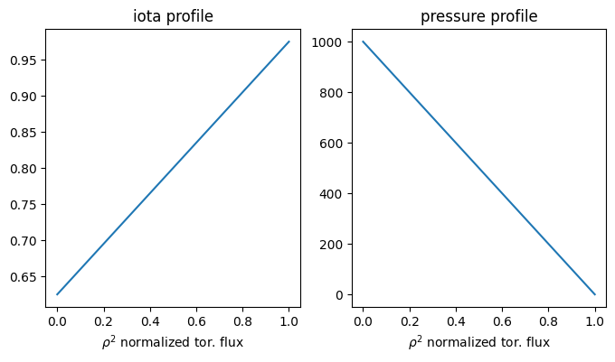
Now, lets visualize the 1D profiles (input quantities) over the radial coordinate \(\rho^2\), which equals the normalized to the toroidal flux \(\Phi / \Phi_\text{edge}\).

fig, ax = plt.subplots(1, 2, figsize=(8, 4))

ax[0].plot(ev.rho**2, ev.iota)
ax[0].set(xlabel="$\\rho^2$ normalized tor. flux", title="iota profile")
ax[1].plot(ev.rho**2, ev.p)
ax[1].set(xlabel="$\\rho^2$ normalized tor. flux", title="pressure profile");

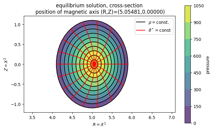
Visualize poloidal plane

As we evaluated on a \(\rho,\vartheta\) grid, we can visualize the poloidal plane (\(\zeta=0\)). Note that contours of pressure, \(\rho\) and of the straight-field line angle \(\theta^* =\theta +\lambda(\theta,\zeta)\) are shown.

fig, ax = plt.subplots(1, 1, figsize=(8, 5))

R = ev.X1[:, :, 0]
Z = ev.X2[:, :, 0]
R_axis = R[0, 0].item()
Z_axis = Z[0, 0].item()
rho_vis = R * 0 + ev.rho
theta_vis = R * 0 + ev.theta
thetastar_vis = ev.LA[:, :, 0] + ev.theta
p_vis = R * 0 + ev.p
rho_levels_vis = np.linspace(0, 1 - 1e-10, 11)
theta_levels_vis = np.linspace(0, 2 * np.pi, 16, endpoint=False)
c = ax.contourf(R, Z, p_vis, alpha=0.75)
fig.colorbar(c, ax=ax, label="pressure")
ax.contour(R, Z, rho_vis, rho_levels_vis, colors="black")
ax.contour(R, Z, thetastar_vis, theta_levels_vis, colors="red")
ax.set(
    xlabel="$R=X^1$",
    ylabel="$Z=X^2$",
    title=f"equilibrium solution, cross-section\n position of magnetic axis (R,Z)=({R_axis:.5f},{Z_axis:.5f})",
    aspect="equal",
    xlim=[0.8 * np.amin(R), 1.2 * np.amax(R)],
    ylim=[1.1 * np.amin(Z), 1.1 * np.amax(Z)],
)
ax.legend(
    handles=[
        plt.Line2D([0], [0], color="black", label="$\\rho=$const."),
        plt.Line2D([0], [0], color="red", label="$\\vartheta^*=$const"),
    ]
);

---

pygvec command line interface

We can also work only on the command line with a parameter file. Lets write the parameters from above to a .toml file using

gvec.util.write_parameters(params, "elliptok_parameters.toml")

and then run pygvec on the command line (with the virtual environment activated) as

mkdir run_02
cp elliptok_parameters.toml run_02/.
cd run_02
export OMP_NUM_THREADS=2
pygvec run elliptok_parameters.toml
cd ..
ls run_02/.

You should then be able to load the state from the runpath as done above:

state = gvec.find_state("run_02")