Frame aligned Poincaré plots

This notebook covers:

• how to obtain frame aligned Poincaré plots (e.g. G-Frame)

• how to use coil-fields with a GVEC state

For the example we use a figure-8 like quasr-case from the vast and excellent quasr-database.

# set the number of OpenMP threads before importing gvec
import os

os.environ["OMP_NUM_THREADS"] = "1"

import numpy as np
import plotly.graph_objects as go
import matplotlib.pyplot as plt

from pathlib import Path
from gvec import Run
from gvec.coils import (
    intersection_planes_from_state,
    trace_fieldlines,
    get_phi_edge_from_coils,
)
from gvec.scripts.quasr import load_quasr, get_coils_from_json_file
from gvec.util import chdir, read_parameters

Setting up the quasr case

To build the quasr case we use the GVEC/QUASR interface, which

• downloads the necessary files,

• builds a suitable G-Frame,

• provides a parameter file.

Also we extract the quasr coils into a GVEC CoilSet. There is a dependency on the simsopt python package to evaluate the objects from the QUASR database.

Note that per default the total toroidal flux \(\phi_{\text{edge}}\) is set to 1 Wb when using the QUASR interface. To get a more realistic value, we can estimate this value from the coil field and the initial equilibrium geometry via the utility function get_phi_edge_from_coils.

# choose a testcase / quasr ID
ID = 189686

# create a corresponding directory
save_path = Path("quasr")
if not save_path.exists():
    save_path.mkdir()
with chdir(save_path):
    # download the quasr case and translate it into a GVEC input file
    load_quasr(ID, tol=1e-4)

    # utility to get the quasr coils into a GVEC CoilSet
    coil_set = get_coils_from_json_file(f"quasr-{ID:07d}.json")

    # run the quasr case with GVEC
    params = read_parameters(f"quasr-{ID:07d}-parameters.toml")

    # increase this tolerance and resolution for more accurate equilibrium results
    params["minimize_tol"] = 1e-4

    # initialize a Run object, this does not yet solve for the equilibrium!
    gvec_run = Run(params, quiet=False)

    # Since we do not know the total toroidal flux we can estimate it from the coil-field
    gvec_run.parameters["PhiEdge"] = get_phi_edge_from_coils(
        gvec_run.state, coil_set
    )

    # to actually run the case uncomment the next line
    # gvec_run.run()

    state = gvec_run.state

Visualizing the 3D geometry

# get the last closed flux surface positions and mod B
ev = state.evaluate(
    "pos",
    "mod_B",
    rho=1.0,
    theta=np.linspace(0, 2 * np.pi, 128),
    zeta=np.linspace(0, 2 * np.pi, 64),
).sel(rho=1.0)

# extract the boundary geometry
boundary = ev.pos


def plot_3d_coils_plus_surface(
    boundary, coil_set, surface_quanitiy, label=None, **kwargs
):
    # visualize the coils
    fig = coil_set.plot(
        show=False,
        line={"color": "black"},
        showlegend=False,
    )
    fig["layout"]["scene"]["aspectmode"] = "data"

    # plot the boundary colored with surface_quanitiy
    fig.add_trace(
        go.Surface(
            x=boundary.sel(xyz="x"),
            y=boundary.sel(xyz="y"),
            z=boundary.sel(xyz="z"),
            surfacecolor=surface_quanitiy,
            colorbar_title_text=label,
            **kwargs,
        )
    )
    return fig


fig3D = plot_3d_coils_plus_surface(
    boundary, coil_set, ev.mod_B, label="B / T"
)
fig3D.show()

Fieldline tracing

• initialize fieldlines on equilibrium flux surfaces by using the pos quantity from an evaluation dataset

• obtain event functions for frame aligned planes via intersection_planes_from_state \(\rightarrow\) frame aligned Poincaré sections

• for more customizable intersection planes use gvec.coils.IntersectionPlane

• for higher resolution plots one can increase the time for which to trace the fieldlines

n_rho = 4  # number of radial starting positions for fieldlines

# zetas where we want to place an intersection plane
zetas = np.linspace(0, 2 * np.pi / state.nfp, 4, endpoint=False)

# initialize the fieldlines on the flux-surfaces
rho = np.linspace(0.01, 1, n_rho)
starts = state.evaluate(
    "pos",
    zeta=0.0,
    theta=0.0,
    rho=rho,
).pos

# define frame aligned intersection planes
planes = intersection_planes_from_state(
    state, zetas=zetas, min_box_size=0.1
)

# perform the fieldline tracing
tree_quasr = trace_fieldlines(
    starts=starts,
    coils=coil_set,
    time=400,  # increase this for better resolution
    events=planes,
    rtol=1e-6,
)

  0%|          | 0/4 [00:00<?, ?it/s]
 25%|██▌       | 1/4 [00:04<00:14,  4.88s/it]
 50%|█████     | 2/4 [00:09<00:09,  4.88s/it]
 75%|███████▌  | 3/4 [00:14<00:04,  4.93s/it]
100%|██████████| 4/4 [00:19<00:00,  5.00s/it]
100%|██████████| 4/4 [00:19<00:00,  4.96s/it]

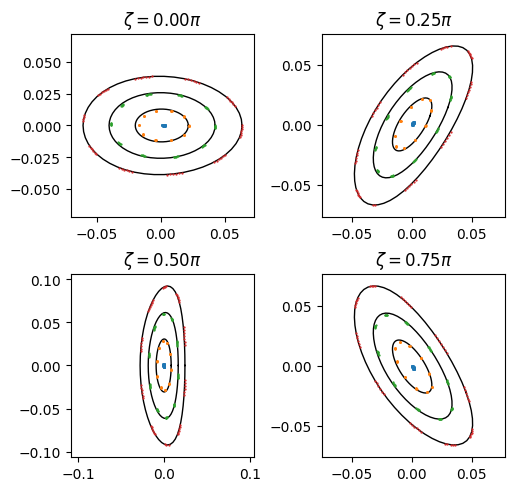
Frame aligned Poincaré plots

• if event functions are generated via intersection_planes_from_state, the returned data-tree has entries for \(X^1\) and \(X^2\)

• new data-tree entries are numbered according to the events list, e.g. event_0_X1 for the first entry of the events list.

• \(\zeta=\) const. cuts of the equilibrium can be obtained via plot_poloidal_plane

theta = np.linspace(0, 2 * np.pi, 128, endpoint=True)
fig, axs = state.plot_poloidal_plane(
    rho_contours=4, zeta=zetas, quantity=None, theta_contours=0
)
axs = axs.flatten()
for fieldline in tree_quasr:
    ds = tree_quasr[fieldline]
    for i, ax in enumerate(axs):
        ax.scatter(
            ds[f"event_{i}_X1"],
            ds[f"event_{i}_X2"],
            marker=".",
            s=1.5,
            zorder=200,
        )

Visualizing fieldlines in 3D

ax3Df = coil_set.plot(
    show=False,
    line={"color": "black"},
    showlegend=False,
)
ax3Df["layout"]["scene"]["aspectmode"] = "data"

for fieldline in tree_quasr:
    # plot the fieldlines
    ds = tree_quasr[fieldline]
    ax3Df.add_trace(
        go.Scatter3d(
            x=ds.pos.sel(xyz="x"),
            y=ds.pos.sel(xyz="y"),
            z=ds.pos.sel(xyz="z"),
            mode="lines",
            opacity=0.01,
            line={"color": "green"},
            showlegend=False,
        )
    )
    # plot the Poincaré section in 3D
    for i in range(len(zetas)):
        ax3Df.add_trace(
            go.Scatter3d(
                x=np.array(ds[f"event_{i}"].sel(xyz="x")),
                y=np.array(ds[f"event_{i}"].sel(xyz="y")),
                z=np.array(ds[f"event_{i}"].sel(xyz="z")),
                mode="markers",
                marker=dict(size=0.5, color="blue"),
                showlegend=False,
            )
        )
ax3Df.show();

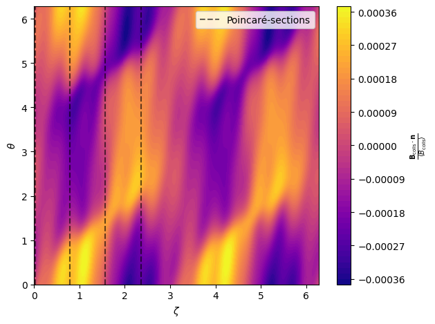
Using equilibrium quantities with coil-fields

• coil-fields can be evaluated at the equilibrium relevant positions using the pos quantity of an equilibrium dataset

• typical postprocessing is possible in this case

• example calculates \(\mathbf{B}_{\text{coils}}\cdot \mathbf{n}\) on the equilibrium boundary (\(\mathbf{n}\) is the surface normal on the boundary)

ev = state.evaluate(
    "pos",
    "normal",
    rho=1.0,
    theta=np.linspace(0, 2 * np.pi, 128),
    zeta=np.linspace(0, 2 * np.pi, 256),
)
n = ev.normal

ev_coils = coil_set.eval_mod_B(ev.pos)

Bdotn = (ev_coils.B * n).sum(dim="xyz")
Bdotn_norm = Bdotn / ev_coils.mod_B.mean()
Bdotn_norm = Bdotn_norm.sel(rho=1.0)

Visualizing \(\mathbf{B}_{\text{coils}}\cdot \mathbf{n}\)

figc, axc = plt.subplots(tight_layout=True)
c = axc.contourf(
    Bdotn_norm.zeta,
    Bdotn_norm.theta,
    Bdotn_norm,
    levels=60,
    cmap="plasma",
)
c_label = r"$\frac{\mathbf{B}_{\text{coils}}\cdot \mathbf{n}}{\langle B_{\text{coils}}\rangle}$"
axc.set(xlabel=r"$\zeta$", ylabel=r"$\theta$")
zetas[0] = 2.5e-2  # shift zeta=0 for better visibility in the plot
axc.vlines(
    zetas,
    0,
    2 * np.pi,
    linestyle="--",
    color="k",
    alpha=0.6,
    label=r"Poincaré-sections",
)
axc.legend()
figc.colorbar(c, label=c_label);

Alternatively we can visualize this also in 3D.

fig3D_BdotN = plot_3d_coils_plus_surface(
    ev.pos.sel(rho=1.0), coil_set, Bdotn.sel(rho=1.0), label="B.n / T"
)
fig3D_BdotN.show()